Turtle Trading System 2: A 20-Year Backtest Across 26 Futures Markets
Quant Trading
A complete 20-year backtest of Turtle System 2 across 26 diversified futures markets — currencies, rates, energies, metals, grains, softs, and livestock. We analyze the system's performance from 2006 to 2026, expose its weaknesses (6 years of stagnation, low Sharpe in bull markets), and introduce the Turtle Overlay: a portfolio construction approach that combines a 75% SPX / 25% Cash base with the Turtle's uncorrelated P&L on top. Full Python implementation included, downloadable Jupyter Notebook.
Antoine
CEO - CodeMarketLabs
2026-04-17
Turtle Trading System 2: A 20-Year Backtest Across 26 Futures Markets
In 1983, Richard Dennis made a bet: anyone could be taught to trade. He recruited 23 people, handed them a simple set of rules, and called them the Turtle Traders. Some went on to generate hundreds of millions of dollars. Forty years later, the question is no longer whether the system worked — it is whether it still works today, and more importantly, how to deploy it in a modern portfolio. This article presents a complete 20-year backtest of Turtle System 2 across 26 diversified futures markets, an honest analysis of its strengths and weaknesses, and three overlay configurations — from a pure cash base to an aggressive 80/20 equity split — to show the full range of what the strategy can do.
What this article covers
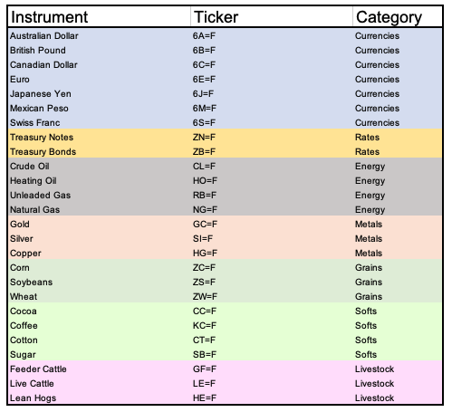
The three rules of Turtle System 2: 55-day breakout entry, 20-day exit, ATR-based position sizing across 26 futures markets.
A full 20-year backtest from 2006 to 2026 on currencies, rates, energies, metals, grains, softs, and livestock.
An honest breakdown of the three overlay strategies: Turtle alone (0/100), Turtle + 60/40, and Turtle + 80/20 — with their exact parameters and results.
Why Strategy 3 (80/20, risk_pct=0.9%) actually beats SPY on this backtest — and what that means in practice.
A full Python implementation on a modular backtesting framework, with equity curve, drawdown panel, and performance dashboard.
A downloadable Jupyter Notebook with the complete code, ready to run on Yahoo Finance data.
1. The Strategy: Three Rules, 26 Markets
Turtle System 2 is a pure trend-following strategy. The rules have been public since the 1990s. Entry triggers when the daily close breaks above the 55-day rolling high (long) or below the 55-day rolling low (short) — using yesterday's high/low with shift(1) to eliminate any look-ahead bias. Exit triggers when the price reverses through the 20-day rolling high or low. Position size is set by the ATR over 20 days: unit_size = (capital × risk_pct) / ATR20. This means each unit risks an identical dollar amount regardless of which market you are trading — a $5 corn move and a $5 crude oil move carry the same weight in the portfolio.
Pyramiding adds up to 3 additional units per market as the trade moves in your favor, each time price advances 0.5 × ATR from the last entry. Each pyramid entry carries its own 2 × ATR stop-loss. The exposure limits prevent concentration: maximum 4 units per market, 6 per category (currencies, metals, energy, etc.), 10 per direction, and 12 total across all 26 markets. The system runs fully automated — no discretionary override.
tableau-tickers-categories-contrats-futures
python
# ── Data download ─────────────────────────────────────────────PERIOD ="20y"EXCLUDE =set()# add names here to exclude specific marketsACTIVE_FUTURES ={k: v for k, v in FUTURES.items()if k notin EXCLUDE}tickers =[v["ticker"]for v in ACTIVE_FUTURES.values()]raw = yf.download(tickers, period=PERIOD, interval="1d", progress=True, auto_adjust=True)["Close"]raw.index = pd.to_datetime(raw.index).tz_localize(None)ticker_to_name ={v["ticker"]: k for k, v in ACTIVE_FUTURES.items()}raw.columns =[ticker_to_name.get(c, c)for c in raw.columns]data = raw.dropna()print(f"Period : {data.index[0].date()} → {data.index[-1].date()}")print(f"Nb Days : {len(data)} | Markets : {len(data.columns)}")# ── SPY and ^IRX (T-bill rate as cash proxy) ──────────────────spx_raw = yf.download("SPY", period=PERIOD, progress=False, auto_adjust=True)["Close"]ifisinstance(spx_raw, pd.DataFrame): spx_raw = spx_raw.iloc[:,0]spx_raw.index = pd.to_datetime(spx_raw.index).tz_localize(None)spx_raw = spx_raw.dropna()cash_raw = yf.download("^IRX", period=PERIOD, progress=False, auto_adjust=True)["Close"]ifisinstance(cash_raw, pd.DataFrame): cash_raw = cash_raw.iloc[:,0]cash_raw.index = pd.to_datetime(cash_raw.index).tz_localize(None)cash_raw = cash_raw.dropna()# ── Align all series on the same trading calendar ─────────────common_start =max(data.index[0], spx_raw.index[0], cash_raw.index[0])data = data[data.index >= common_start]spx = spx_raw.reindex(data.index, method="ffill")irx = cash_raw.reindex(data.index, method="ffill").fillna(0)daily_rfr = irx /100/252# annualised % → daily rateprint(f"Aligned Period : {data.index[0].date()} → {data.index[-1].date()}")
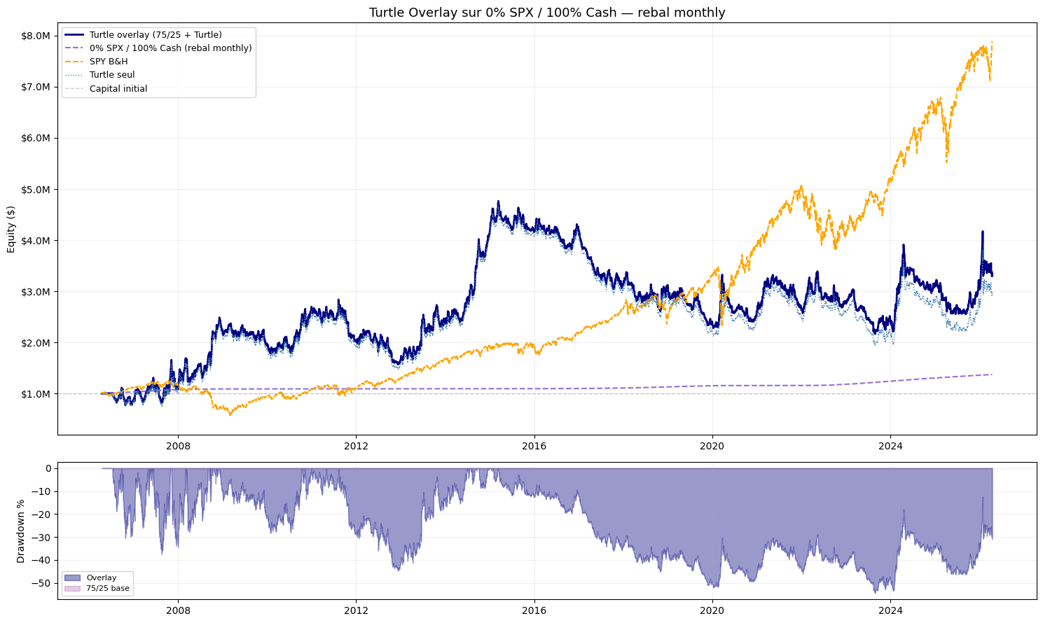
2. Strategy 1 — Turtle Alone (0% SPX / 100% Cash)
The baseline: $1,000,000 sits entirely in cash (T-bill rate via ^IRX), and the Turtle runs on top using futures margins only. No equity exposure whatsoever. This is the purest read of the system — trend-following P&L plus risk-free cash return, nothing else.
The first decade tells a compelling story. In 2008, while SPY loses 50%, the Turtle shorts falling markets and goes long rising bonds — it makes money. The equity curve climbs steadily to near $3M by 2014. Then reality hits: from 2015 to 2020, the system stagnates for nearly six years. Low-volatility macro, range-bound commodities, near-zero rates — exactly the conditions that kill trend-following. The curve goes flat while SPY gains 150%. This is not a bug. It is the structural cost of a strategy that needs big, sustained moves to survive. The question is not whether it recovers — it does. The question is whether you hold through six years of underperformance without cutting it at the worst moment.
turtle-overlay-suivi-de-tendance-pur
python
# ── Strategy 1 parameters ─────────────────────────────────────INITIAL_CAP =1_000_000W_SPX =0.0# 0% in SPYW_CASH =1- W_SPX # 100% in cash (^IRX)REBAL_FREQ ="monthly"TURTLE_SYSTEM =2# System 2 = 55-day breakoutTURTLE_RISK_PCT =0.0050# 0.5% of capital risked per unit# ── Base portfolio (pure cash) ────────────────────────────────base = compute_basis_portfolio(spx, daily_rfr, INITIAL_CAP, w_spx=W_SPX, rebal_freq=REBAL_FREQ)print(f"Base portfolio final value : ${base.iloc[-1]:,.0f}")# ── Run Turtle ────────────────────────────────────────────────engine = SpotPricingEngine(data)bt = TurtleStrategy(data=data, initial_capital=INITIAL_CAP, system=TURTLE_SYSTEM, risk_pct=TURTLE_RISK_PCT, futures_dict=ACTIVE_FUTURES)turtle_equity = bt.run(data, engine, verbose=False)["equity"]# ── Overlay: base + incremental Turtle P&L ───────────────────turtle_pnl = turtle_equity - INITIAL_CAP
combined = base + turtle_pnl.reindex(base.index, method="ffill").fillna(0)# ── Metrics ───────────────────────────────────────────────────spx_full =(spx / spx.iloc[0])* INITIAL_CAP
print(f"\n{'='*65}")dd_base = metrics(base, INITIAL_CAP,"0% SPX / 100% Cash (base)")dd_turtle = metrics(turtle_equity, INITIAL_CAP,"Turtle alone")dd_combined = metrics(combined, INITIAL_CAP,"Turtle Overlay on 0/100")_ = metrics(spx_full, INITIAL_CAP,"SPY B&H")print(f"{'='*65}")
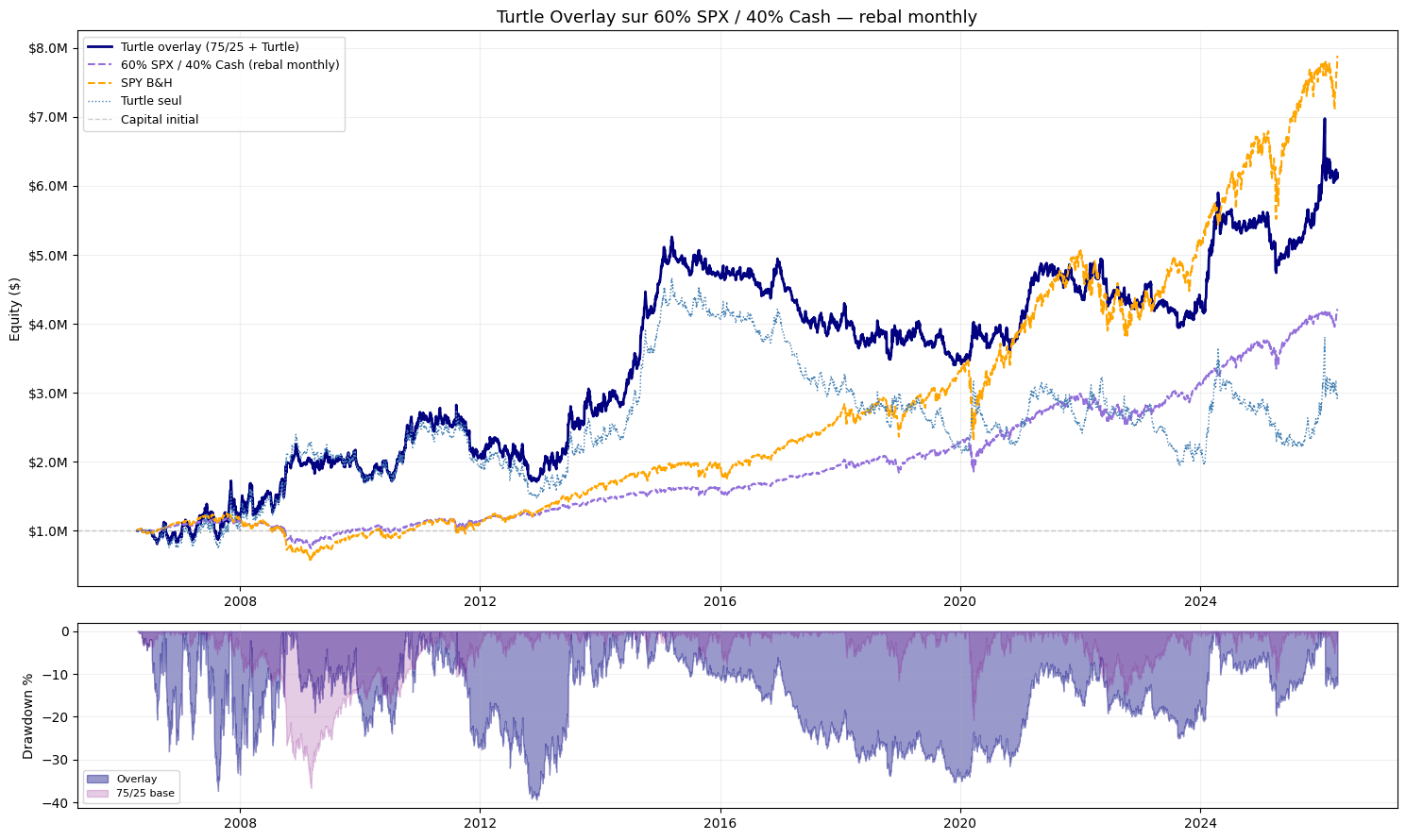
3. Strategy 2 — Turtle + 60/40
The classic institutional allocation — 60% SPY, 40% cash — with the Turtle running on top. The Turtle still uses only futures margin capital, so the 40% cash buffer is more than enough to cover it. The key insight: you are not choosing between the equity allocation and the Turtle. The futures margin requirement leaves the vast majority of capital free to invest elsewhere. This is the Portable Alpha concept in practice.
The 60/40 overlay absorbs the 2008 and 2020 crashes better than pure SPY buy-and-hold, because the Turtle is long on the instruments that rise during those crises — bonds, gold, short equity futures. In the 2015–2020 flat period for the Turtle, the 60% SPY allocation keeps the portfolio moving forward. The result is a smoother equity curve than either strategy alone, with a Sharpe that justifies the added complexity.
turtle-overlay-60-spx-40-cash
python
# ── Strategy 2 parameters ─────────────────────────────────────INITIAL_CAP =1_000_000W_SPX =0.6# 60% in SPYW_CASH =1- W_SPX # 40% in cashREBAL_FREQ ="monthly"TURTLE_SYSTEM =2TURTLE_RISK_PCT =0.0050# same 0.5% risk per unit as Strategy 1base = compute_basis_portfolio(spx, daily_rfr, INITIAL_CAP, w_spx=W_SPX, rebal_freq=REBAL_FREQ)print(f"Base portfolio final value : ${base.iloc[-1]:,.0f}")engine = SpotPricingEngine(data)bt = TurtleStrategy(data=data, initial_capital=INITIAL_CAP, system=TURTLE_SYSTEM, risk_pct=TURTLE_RISK_PCT, futures_dict=ACTIVE_FUTURES)turtle_equity = bt.run(data, engine, verbose=False)["equity"]turtle_pnl = turtle_equity - INITIAL_CAP
combined = base + turtle_pnl.reindex(base.index, method="ffill").fillna(0)spx_full =(spx / spx.iloc[0])* INITIAL_CAP
print(f"\n{'='*65}")dd_base = metrics(base, INITIAL_CAP,"60% SPX / 40% Cash (base)")dd_turtle = metrics(turtle_equity, INITIAL_CAP,"Turtle alone")dd_combined = metrics(combined, INITIAL_CAP,"Turtle Overlay on 60/40")_ = metrics(spx_full, INITIAL_CAP,"SPY B&H")print(f"{'='*65}")
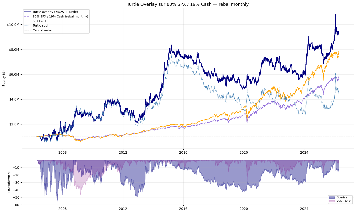
4. Strategy 3 — Turtle + 80/20 (Aggressive)
Strategy 3 pushes the equity weight to 80% and raises the Turtle risk per unit to 0.9% — nearly double Strategy 2. The thinner 20% cash buffer means less room for margin calls, so the higher risk_pct compensates by sizing positions more aggressively on the available capital. This is the version that, on this 20-year backtest, ends up beating SPY buy-and-hold in absolute return.
A word of honesty: beating SPY over a specific 20-year window does not mean this configuration will always win. The 0.9% risk per unit produces larger drawdowns when the Turtle is wrong, and those drawdowns compound on top of the equity drawdown from the 80% SPX allocation. The 2008 period is particularly brutal for this configuration. The outperformance is real on this backtest, but the path to get there is significantly rougher than pure SPY. The Sharpe is lower, and the maximum drawdown is higher. It is a higher-volatility, higher-return profile — not a free lunch.
turtle-overlay-80-spx-20-cash
python
# ── Strategy 3 parameters ─────────────────────────────────────INITIAL_CAP =1_000_000W_SPX =0.8# 80% in SPYW_CASH =1- W_SPX # 20% in cashREBAL_FREQ ="monthly"TURTLE_SYSTEM =2TURTLE_RISK_PCT =0.00900# 0.9% — more aggressive to compensate the thinner cash bufferbase = compute_basis_portfolio(spx, daily_rfr, INITIAL_CAP, w_spx=W_SPX, rebal_freq=REBAL_FREQ)print(f"Base portfolio final value : ${base.iloc[-1]:,.0f}")# Pure cash benchmark for the performance dashboardrfr = compute_basis_portfolio(spx, daily_rfr, INITIAL_CAP, w_spx=0, rebal_freq=REBAL_FREQ)engine = SpotPricingEngine(data)bt = TurtleStrategy(data=data, initial_capital=INITIAL_CAP, system=TURTLE_SYSTEM, risk_pct=TURTLE_RISK_PCT, futures_dict=ACTIVE_FUTURES)turtle_equity = bt.run(data, engine, verbose=False)["equity"]turtle_pnl = turtle_equity - INITIAL_CAP
combined = base + turtle_pnl.reindex(base.index, method="ffill").fillna(0)spx_full =(spx / spx.iloc[0])* INITIAL_CAP
print(f"\n{'='*65}")dd_base = metrics(base, INITIAL_CAP,"80% SPX / 20% Cash (base)")dd_turtle = metrics(turtle_equity, INITIAL_CAP,"Turtle alone")dd_combined = metrics(combined, INITIAL_CAP,"Turtle Overlay on 80/20")_ = metrics(spx_full, INITIAL_CAP,"SPY B&H")print(f"{'='*65}")
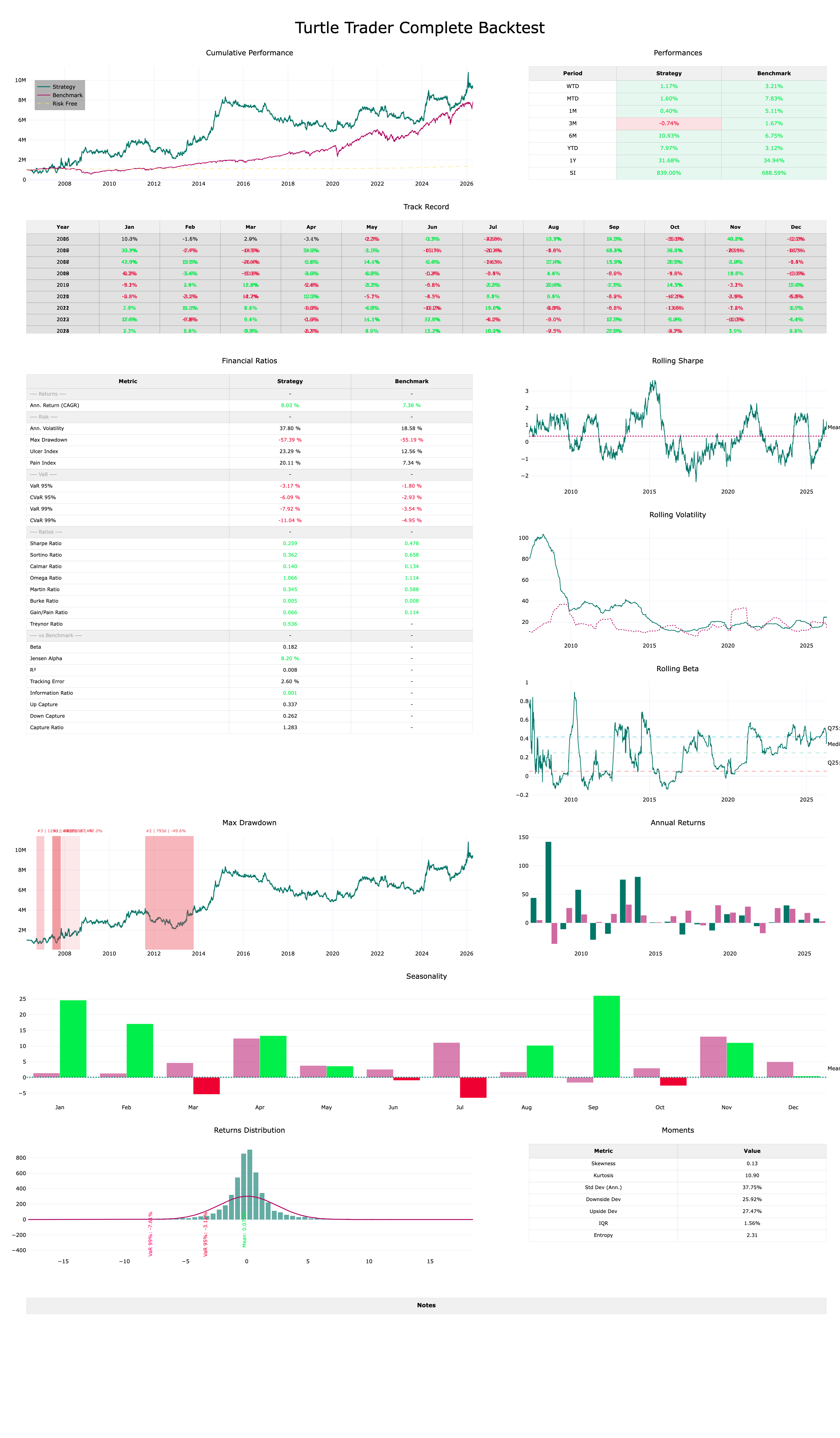
5. Full Performance Dashboard
The final cell of the notebook assembles a full performance dashboard via the equity_curve library, using the Strategy 3 comparison DataFrame. It produces rolling CAGR, rolling Sharpe, rolling volatility, correlation matrix, and the top 3 drawdown periods highlighted — everything you need to evaluate whether the combined strategy holds up beyond the simple equity curve comparison.
tableau-de-bord-analytique-backtest-complet
python
from equity_curve.graphs import dashboard
from equity_curve.performances import Performances
from equity_curve.utils.financial_ts import PortfolioTs
# Build the comparison DataFrame — Strategy 3 contextcomparison = pd.DataFrame({"strategy": combined,# Turtle overlay on 80/20"base_75_25": base,# base 80/20 without Turtle"turtle": turtle_equity,# Turtle alone"benchmark": spx_full,# SPY B&H"risk_free": rfr,# pure cash (^IRX)}, index=base.index)print("\nLast 5 rows:")print(comparison.tail(5).to_string())portfolio = PortfolioTs(comparison)perf = Performances( strat=portfolio, computation_date=datetime(2026,4,16), period_per_year=252)fig = dashboard( perf, window_roll=180,# 180-day rolling window top_dd=3,# highlight top 3 drawdown periods mode='dark', title='Global Portfolio Strategy')fig.show()
6. Three Strategies, One Conclusion
The three strategies answer different questions. Strategy 1 (0/100) asks: how does the Turtle perform in complete isolation? The answer is: well in crisis regimes, poorly in prolonged bull markets, and with a Sharpe that is hard to justify as a standalone allocation. Strategy 2 (60/40) asks: can the Turtle improve a classic balanced portfolio? The answer is yes — smoother drawdowns in 2008 and 2020, better risk-adjusted returns over the full period, and only a marginal cost during the 2015–2020 flat stretch. Strategy 3 (80/20, risk_pct=0.9%) asks: what happens if you maximize both the equity beta and the trend-following exposure? The answer is a configuration that outperforms SPY in absolute return on this backtest — but with higher drawdown, lower Sharpe, and a much more demanding psychological profile.
The practical takeaway is not that Strategy 3 is superior. It is that the Turtle Overlay is a flexible tool — the W_SPX and TURTLE_RISK_PCT parameters let you dial the tradeoff between equity-like returns and crisis protection anywhere on the spectrum. The notebook makes it trivial to re-run all three configurations and compare them directly.
Image non trouvée (ID: youtube_thumbnail_clickable)
Download the Jupyter Notebook
The complete backtest is available as a Jupyter Notebook. It includes the full TurtleStrategy implementation, all three overlay strategies with their exact parameter blocks, equity curve and drawdown computation, and the full performance dashboard. The code runs directly on Yahoo Finance data — no data subscription required. Change W_SPX, TURTLE_RISK_PCT, or REBAL_FREQ and re-run any strategy in seconds.
What the Notebook contains
Full TurtleStrategy class: 55-day breakout, 20-day exit, ATR-based sizing, pyramiding up to 4 units, and exposure limits enforced on every bar.
Three complete strategy blocks: Turtle alone (0/100, risk_pct=0.5%), Turtle + 60/40 (risk_pct=0.5%), and Turtle + 80/20 (risk_pct=0.9%).
Base portfolio function: configurable SPX weight and rebalancing frequency — monthly, quarterly, or yearly.
Performance dashboard via equity_curve: rolling CAGR, Sharpe, volatility, top drawdown highlights, and correlation matrix.
Ready to run on Yahoo Finance data — 20 years, 26 markets, no proprietary data feed needed.
What are the exact entry and exit rules of Turtle System 2?
Entry is triggered when the daily close breaks above the 55-day rolling high (long) or below the 55-day rolling low (short). Both use shift(1) on the rolling window to avoid look-ahead bias — today's signal is always based on yesterday's levels. Exit is triggered when the price reverses through the 20-day rolling high (for shorts) or low (for longs). Position size is computed as (capital × risk_pct) / ATR20, where ATR20 is the 20-day average of the absolute daily price change.
Why is the risk_pct different between Strategy 2 (0.5%) and Strategy 3 (0.9%)?
Strategy 3 allocates only 20% of capital to cash, compared to 40% in Strategy 2. With less cash buffer available for futures margins, the position sizing needs to be more aggressive on the capital that is deployed in the Turtle to generate a meaningful overlay contribution. The 0.9% risk_pct roughly compensates for the reduced margin capital while keeping the absolute dollar risk per unit in a similar range.
Strategy 3 beats SPY on this backtest — does that mean it is the best strategy?
Not necessarily. The 20-year window includes two major crises (2008, 2020) where the Turtle contributes significantly, and that boosts the long-term return of the 80/20 overlay above SPY. But Strategy 3 also has a higher maximum drawdown and a lower Sharpe ratio than SPY over the same period. It wins in absolute return while losing in risk-adjusted return. Whether that is a good tradeoff depends entirely on your ability to hold through large, extended drawdowns without abandoning the strategy.
What is the Portable Alpha concept, and why does it matter here?
Portable Alpha refers to separating alpha generation from beta exposure. Futures contracts only require 10–20% of their notional value as margin. A $1,000,000 account running the Turtle on 26 markets uses roughly $150,000–$200,000 in margin at any given time. The remaining capital can be invested in SPY without any conflict. The Turtle P&L is simply added on top of the base portfolio equity series. You get the equity beta and the trend-following alpha from the same capital pool.
Why does the system stagnate from 2015 to 2020?
Trend-following systems require sustained, directional moves across markets. The 2015–2020 period combined low macro volatility, range-bound commodity markets, and near-zero interest rates that suppressed trends in currencies and rates. The system generated frequent false breakouts — entries that reversed quickly and hit the 20-day exit stop at a small loss. This is the structural cost: lose small on many trades, win large on the rare sustained trends. When trends are absent across all 26 markets simultaneously, costs accumulate and the equity curve goes flat.
Can I change the markets or parameters in the notebook?
Yes. Each strategy block exposes TURTLE_SYSTEM (1 or 2), TURTLE_RISK_PCT, W_SPX, and REBAL_FREQ as top-level variables. You can add markets to the FUTURES dictionary using any Yahoo Finance futures ticker, or exclude specific markets by adding their name to the EXCLUDE set. Changing REBAL_FREQ from monthly to yearly has a meaningful effect on the base portfolio returns and is worth exploring.
Does the backtest account for transaction costs?
Yes — a fixed $2 fee is applied at entry and exit for every trade signal. This approximates institutional round-trip commissions. Bid-ask spread and futures roll slippage are not modeled. Roll costs are implicitly absorbed by Yahoo Finance's continuous adjusted price series, though for less liquid contracts like Lean Hogs or Cocoa the real-world slippage would be higher than what the backtest captures.