Reconstructing 20 Years of Volatility: GARCH, SVI and the VRP — A Practical Guide for Options Backtesting
Quant Trading
How to reconstruct a complete historical volatility surface from scratch using only daily price data — no options data subscription required. We cover the Variance Risk Premium (VRP), GARCH(1,1) conditional volatility estimation with Student-t innovations, and the SVI parameterization for arbitrage-free volatility smiles. Includes regime-dependent skew calibration (crisis vs calm), the complete QuantSkewEngine Python class, and a skew timeline visualization across 20 years of market regimes.
Antoine
CEO - CodeMarketLabs
2026-04-28
Reconstructing 20 Years of Volatility: GARCH, SVI, and the VRP — A Practical Guide for Options Backtesting
Backtesting an options strategy sounds straightforward until you face the real problem: you need implied volatility data for every strike, every day, going back 20 years. Professional data providers charge thousands of dollars per year for that. Historical options chains from CBOE or OptionMetrics cost even more. For most independent quants and systematic traders, that data simply does not exist. This article shows a complete, reproducible approach to reconstructing a volatility surface from scratch — using only daily price data from Yahoo Finance — and explains the theoretical foundations behind each step: what the Variance Risk Premium is, why GARCH captures realized volatility better than a simple rolling window, and how the SVI parameterization produces a realistic implied volatility smile across strikes and regimes.
What this article covers
What the Variance Risk Premium (VRP) is and why it is the theoretical foundation of short-volatility strategies.
Why realized volatility alone is not enough to price options — and what implied volatility adds.
GARCH(1,1) with Student-t innovations: the standard model for conditional volatility estimation on equity indices.
The SVI (Stochastic Volatility Inspired) parameterization: a 5-parameter model that produces arbitrage-free volatility smiles.
Regime-dependent skew: how to calibrate sigma_smooth, rho, skew_strength, and m dynamically based on the volatility level.
The complete QuantSkewEngine class: from raw price data to a full interpolated surface for every trading day.
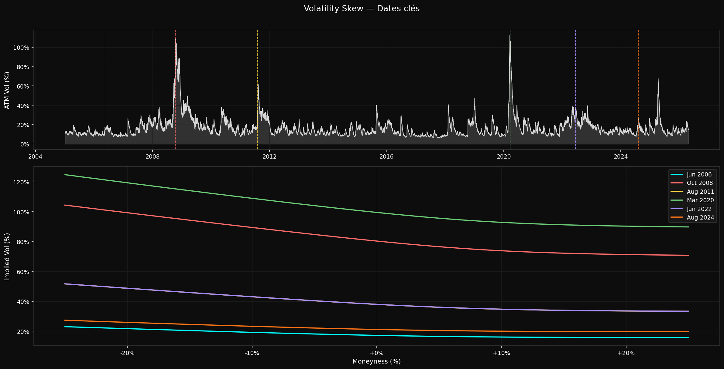
Visualization: a skew timeline chart showing how the smile deforms across crisis and calm regimes.
Next step: what calibrating on actual implied vol data would look like, and why the synthetic surface is a defensible approximation.
1. The Variance Risk Premium: Why Selling Volatility Works
The Variance Risk Premium (VRP) is the difference between implied volatility and subsequently realized volatility. On equity indices, implied vol — the vol priced into options by the market — has historically been higher than the vol that actually materialized over the same period. The VIX, for instance, has averaged around 19–20% over the past 30 years, while the actual realized volatility of the S&P 500 has averaged closer to 15–16%. That gap — roughly 3 to 5 vol points on average — is the VRP. It represents the risk premium that option buyers pay for protection, and that option sellers collect in exchange for bearing tail risk.
The VRP is not constant. It compresses in calm regimes (2013–2017) and explodes during stress — in March 2020, the VIX spiked to 85 while realized vol over the same 30 days was closer to 60%. The spread between the two is what drives the P&L of systematic short-volatility strategies. When the VRP is positive and stable, selling options collects premium consistently. When the VRP collapses or reverses — as it can during sharp, fast dislocations — short volatility positions bleed.
In a backtest without implied vol data, the VRP is the key parameter you need to model. The vrp_bps parameter in the QuantSkewEngine does exactly this: it adds a fixed basis point spread on top of the GARCH-estimated realized vol to approximate the implied vol level the market would have priced. Setting vrp_bps=0 means you assume no VRP — a conservative assumption. Setting vrp_bps=300 adds 3 vol points, which is close to the long-run historical average. This is the most honest lever in the entire engine: it controls the gap between what the model thinks realized vol is, and what it assumes the market would have charged.
2. From Realized to Implied: Why You Need a Model
Realized volatility — the standard deviation of daily log-returns over a rolling window — is backward-looking by construction. It tells you what happened. Options are priced on what the market expects to happen. This distinction matters for backtesting. If you price options using a simple 20-day or 30-day rolling realized vol, you will systematically underprice options in calm regimes (when realized vol is low but the market still charges a fear premium) and overprice them after a crisis (when realized vol is high but the market has already repriced lower).
A conditional volatility model — specifically GARCH — partially solves this problem. GARCH(1,1) estimates volatility as a weighted average of the long-run variance, the previous period's squared return, and the previous period's estimated variance. It mean-reverts. After a spike, it decays back toward the unconditional mean faster than a simple rolling window. After a period of calm, it stays low rather than being dragged up by a 30-day window that includes a distant crisis. This makes GARCH-estimated vol a better proxy for what the market would have priced — not perfect, but directionally correct.
The Student-t distribution for innovations matters on equity indices. Daily returns are fat-tailed — extreme moves happen more often than a Gaussian model predicts. Fitting GARCH with Student-t innovations produces a better in-sample fit and, more importantly, better-calibrated volatility estimates during the tail events that drive most of the P&L in options strategies. The degrees-of-freedom parameter of the t-distribution is estimated jointly with the GARCH parameters during the fit.
3. The SVI Model: A Realistic Volatility Smile
Black-Scholes assumes constant volatility across strikes. The market does not. Out-of-the-money puts on equity indices trade at significantly higher implied vols than at-the-money options — this is the volatility skew. Far OTM calls trade at lower vols than ATM. The result is a smile (or more precisely, a smirk) when you plot implied vol against strike or log-moneyness.
The SVI parameterization, introduced by Gatheral (2004), describes the total implied variance w(k) = σ²(k) × T as a function of log-moneyness k = log(K/F): w(k) = a + b × (ρ × (k − m) + √((k − m)² + σ²)). The five parameters have intuitive interpretations: a controls the overall level of variance (the ATM point), b controls the slope and curvature, ρ is the correlation between spot and vol (negative for equity indices — the leverage effect), m shifts the minimum of the smile away from ATM, and σ (sigma_smooth here) controls the smoothness of the transition from the put wing to the call wing. A small sigma_smooth produces a sharp V-shape; a large one produces a smooth U-shape.
The key property of SVI is that it is arbitrage-free by construction for a wide range of parameters — specifically, it satisfies the no-butterfly-arbitrage condition that prevents calendar spread or butterfly arbitrage from appearing in the surface. This makes it appropriate for use in a pricing engine: you will not generate negative option prices or inverted spreads simply by evaluating the surface at different strikes.
4. Regime-Dependent Parameters: Calibrating the Skew to Market Reality
A single set of SVI parameters cannot capture the behavior of the volatility smile across all market regimes. In calm markets (VIX < 15), the skew is shallow — the difference between 90% and 100% moneyness implied vol might be 3 to 5 vol points. In a crisis (VIX > 40), the same distance can be 20 to 30 vol points. The smile also sharpens — sigma_smooth decreases — and the minimum shifts further toward OTM calls as demand for put protection overwhelms the market.
The QuantSkewEngine handles this through get_skew_params, which maps the GARCH-estimated ATM vol to a set of SVI parameters. Three regimes are defined: crisis (atm_vol > 40%), moderate stress (25–40%), and calm (< 25%). In the crisis regime, rho is pushed to −0.99 (almost fully negative correlation between spot and vol moves), skew_strength is 1.2 (steep put wing), m shifts the minimum to 0.08 in log-moneyness space (well into OTM call territory), and sigma_smooth is kept at 0.10 (tight but not singular transition). In the calm regime, all parameters relax toward a shallow, centered smile.
This is a synthetic calibration — the parameters are not fitted to market data but set by hand to match the qualitative shape of the smile in each regime. It is a simplification. But it is a principled one: the direction of every parameter adjustment is grounded in what equity index vol surfaces actually look like. A crisis SPX surface from March 2020 had rho close to −1, a steep put wing, and a minimum well above ATM. The synthetic surface captures this qualitative behavior even without market data to fit it precisely.
5. The Complete QuantSkewEngine
The engine takes a DataFrame with a Close column and builds a complete volatility surface for every trading day. The workflow is: fit one GARCH model on the full return series to extract conditional vol, then generate an SVI surface for each date using the ATM vol from GARCH and the regime-dependent SVI parameters. The result is a dictionary of interpolators — one per date — that can be queried at any strike with get_vol_at_date.
python
import numpy as np
import pandas as pd
from arch import arch_model
from scipy.interpolate import interp1d
from datetime import datetime
import bisect
classQuantSkewEngine:def__init__(self, df): self.df = df
self.surfaces ={} self.returns =100* np.log(self.df['Close']/ self.df['Close'].shift(1)).dropna()defget_skew_params(self, atm_vol):"""Regime-dependent SVI parameters.
Crisis : steep put skew, sharp transition, high skew_strength
Stress : moderate skew
Calm : shallow, centered smile
"""if atm_vol >0.40:# Crisisreturndict(sigma_smooth=0.10, rho=-0.99, skew_strength=1.2, m=0.08)elif atm_vol >0.25:# Moderate stressreturndict(sigma_smooth=0.12, rho=-0.90, skew_strength=0.8, m=0.06)else:# Calmreturndict(sigma_smooth=0.15, rho=-0.75, skew_strength=0.4, m=0.04)defgenerate_surface(self, atm_vol, spot, vrp_bps, skew_strength):"""Build an SVI interpolator for a single date.
vrp_bps : basis points added to ATM vol to approximate the VRP
""" atm_vol_q = atm_vol +(vrp_bps /10000)# add VRP spread ratios = np.linspace(0.70,1.30,101) k = np.log(ratios)# log-moneyness grid p = self.get_skew_params(atm_vol) a = atm_vol_q **2 b = p['skew_strength']* atm_vol_q
defsvi_curve(k_val): k_shifted = k_val - p['m'] total_var = a + b *( p['rho']* k_shifted
+ np.sqrt(k_shifted **2+ p['sigma_smooth']**2))return np.sqrt(max(0.0025, total_var))# floor at 5% vol vols = np.array([svi_curve(val)for val in k])return interp1d(spot * ratios, vols, kind='cubic', fill_value='extrapolate')defrun_backtest_interpolation(self, vrp_bps=0, skew_strength=0.20):"""Fit GARCH once on the full series, then generate a surface for every date.
Note: global GARCH fit uses future data for parameter estimation.
This is a known simplification — parameters are stable and the
impact on conditional vol estimates is small in practice.
""" model = arch_model(self.returns, p=1, q=1, vol='GARCH', dist='t') res = model.fit(disp='off')# Annualised conditional vol vols_annuelles =(res.conditional_volatility /100)* np.sqrt(252)for date, atm_vol in vols_annuelles.items(): clean_date = date.to_pydatetime() spot =float(self.df.loc[date,'Close']) interp = self.generate_surface(atm_vol, spot, vrp_bps, skew_strength) self.surfaces[clean_date]={'spot': spot,'atm_vol': atm_vol,'interpolator': interp
}print(f'Surface generated for {len(self.surfaces)} days.')return self.surfaces
defget_vol_at_date(self, target_date, strike):"""Query the surface at a given strike. Falls back to the nearest
available date if the exact date is missing."""ifhasattr(target_date,'to_pydatetime'): target_date = target_date.to_pydatetime()if target_date in self.surfaces: vol =float(self.surfaces[target_date]['interpolator'](strike))returnmax(0.01, vol)# floor at 1% available =sorted(self.surfaces.keys())ifnot available:return0.15 idx = bisect.bisect_right(available, target_date)-1 vol =float(self.surfaces[available[max(0, idx)]]['interpolator'](strike))returnmax(0.01, vol)
6. Visualizing the Surface: A Skew Timeline
The most useful diagnostic for the engine is a skew timeline: plot the volatility smile at several key dates on the same chart, with the ATM vol series above for context. This immediately shows whether the regime-dependent calibration is working — crisis dates should have steep put wings, calm dates should have shallow symmetric smiles.
7. Limitations and the Path to a Properly Calibrated Surface
The synthetic surface has three honest limitations. First, the SVI parameters are not fitted to market data — they are set by hand based on qualitative regime behavior. This means the smile shape is plausible but not accurate. On any given day, the actual market-implied skew at a specific strike may differ significantly from what the engine produces. Second, there is no term structure: the surface does not vary by expiry. A 7-DTE surface should be steeper than a 30-DTE surface; the engine produces the same smile for both. Third, the GARCH model is fitted on the full historical series — a global fit that technically uses future data for parameter estimation. The conditional vol series is not affected much in practice, but it is a known methodological simplification.
The next step toward a properly calibrated surface would be: obtain historical options data (CBOE DataShop, OptionMetrics, or Interactive Brokers historical data for recent periods), extract implied vols at each strike and expiry using a numerical Black-Scholes inversion, and fit the SVI parameters on each date by minimizing the squared error between model and market vols. This would replace the synthetic get_skew_params calibration with a data-driven one, and would immediately expose the term structure. For a first-pass backtest, the synthetic approach is defensible. For production deployment or precise P&L attribution, the calibrated surface is essential.
What the Notebook contains
Complete QuantSkewEngine class with GARCH fit, regime-dependent SVI surface generation, and strike interpolation.
plot_skew_timeline function: ATM vol series (log scale) + smile curves at user-defined dates.
Integration example: how to pass the engine to BSOptionPricingEngine for live option repricing during a backtest.
VRP sensitivity analysis: run the engine at vrp_bps = 0, 150, 300 and compare the resulting option prices.
Ready to run on any Yahoo Finance equity or futures ticker — change the Close column and re-run.
Why use GARCH instead of a simple 30-day rolling volatility?
A rolling window weights all observations equally over the window and ignores everything outside it. GARCH weights recent observations more heavily through its autoregressive structure, and it mean-reverts — after a spike, it decays faster than a 30-day window that will keep the spike in the average for a full month. For options pricing, GARCH also produces smoother transitions between regimes, which avoids the artificial discontinuities that appear when a crisis observation enters or exits a rolling window.
What is the vrp_bps parameter doing exactly?
It adds a fixed number of basis points to the GARCH-estimated ATM vol before generating the SVI surface. vrp_bps=0 means the model assumes implied vol equals realized vol — no risk premium. vrp_bps=300 adds 3 vol points, approximating the historical long-run average VRP on US equity indices. This parameter directly affects option prices: higher vrp_bps means more premium collected on short options and more premium paid on long options. It is the most sensitive parameter in the engine for P&L purposes.
Why does the skew steepen in a crisis?
Demand for OTM put options spikes during market stress. Investors and funds buy puts to hedge long equity exposure, and dealers who sell those puts demand higher premiums to compensate for the increased gap risk. This demand imbalance pushes OTM put implied vols well above ATM vol, steepening the left side of the smile. Simultaneously, OTM call demand decreases as upside speculation drops, flattening the right side. The result is the asymmetric smirk characteristic of equity index surfaces during crises.
What does the m parameter in SVI control?
m shifts the minimum of the variance curve away from the ATM point (k=0 in log-moneyness space). On equity indices, the minimum of the smile is typically slightly above ATM — around 5 to 10% OTM call — because call skew is positive while put skew is negative. Setting m=0.06 to 0.08 shifts the minimum to approximately the 106–108% strike level, which matches observed SPX surfaces well.
Is the global GARCH fit a problem for the backtest?
In principle, yes — fitting GARCH on the full series uses future data to estimate parameters. In practice, GARCH parameters (omega, alpha, beta) are stable and converge quickly on 2–3 years of data. The difference between a global fit and a rolling expanding-window fit is small for the conditional vol series. It would matter more for a strategy that explicitly trades GARCH parameter changes (e.g., a volatility regime-switching strategy). For an Iron Condor backtest where the key driver is premium collection, the approximation is acceptable.
How would you calibrate the surface on real implied vol data?
The process is: for each historical date, collect the market-implied vols at multiple strikes from actual options chains. Convert each (strike, market implied vol) pair to total implied variance w = σ² × T. Then minimize the sum of squared errors between the SVI model w(k) and the market w values, with respect to the five SVI parameters (a, b, rho, m, sigma). This is a nonlinear least squares problem that scipy.optimize.minimize handles well with a good initialization. The resulting parameters replace the hand-calibrated get_skew_params values with data-fitted ones.