Iron Condor Backtest on ES Futures: +1539% in 20 Years — VRP, Greeks, and Honest Limits

In 2003, a systematic options strategy was already quietly compounding on ES Futures. Twenty years later, the numbers tell a clear story: +1539% total return, a Sharpe ratio of 1.14, and a maximum drawdown of −28.4% — against the S&P 500's −57% during the GFC. This article walks through exactly how this Iron Condor backtest was built: the volatility surface reconstruction, the signal logic, the reinvestment scenarios, and — critically — where the model is too generous with itself.

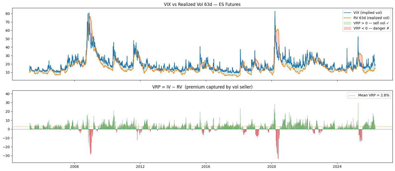
The Volatility Risk Premium (VRP) is the difference between implied volatility and subsequently realized volatility. On equity indices, implied vol — the vol priced into options — has historically been higher than the vol that actually materialized. The VIX has averaged around 19–20% over the past 30 years, while the realized volatility of the S&P 500 has averaged closer to 15–16%. That gap of roughly 3 to 5 vol points is the VRP. It is the risk premium that option buyers pay for protection, and that option sellers collect in exchange for bearing tail risk.

The VRP is not constant. It compresses in calm regimes (2013–2017, late 2024) and explodes during stress — in March 2020, the VIX hit 85 while realized vol over the same 30 days was closer to 60%. In April 2025, the market rallied 7–10% in a single session — a move the implied vol was not pricing. That is exactly the kind of regime where this strategy loses. When the VRP is positive and stable, selling options collects premium consistently. When it collapses or inverts — as it can during fast, sharp dislocations — short volatility positions bleed.

On the chart below, green zones show periods where VRP was positive — the structural edge of the strategy. Red zones show inversions: the realized vol exploded past the implied vol, and any short-vol position was on the wrong side of the trade.

Not all market environments are favorable for selling volatility. Three regimes matter: range markets with low realized vol, where the Iron Condor collects theta without being touched; trending bull markets, where the strategy needs active delta hedging to stay directionally neutral; and crisis or vol-spike regimes, where selling should stop entirely — or positions should be closed.

A simple heuristic: use VIX percentile over the trailing 12 months. If VIX is above the 50th percentile, the premium is sufficient to justify opening positions. Below the 25th percentile, the credit collected is too thin relative to the gamma risk taken. In 2017, the VIX traded below 10 for extended stretches — a regime where the VRP was structurally compressed and most short-vol strategies had minimal edge.

Selling an Iron Condor creates a specific risk profile that can be fully described by five Greeks. Understanding each one is not optional — it is the difference between managing the position and being surprised by it.

Delta (~0 at entry) measures the directional exposure. The goal of the Iron Condor is to stay delta-neutral. At entry, the short call spread and short put spread offset each other. Delta is the number to watch and rebalance continuously — via long or short ES futures — as the market moves. Gamma (negative) is the enemy. It measures how fast your delta moves when the underlying moves. Being short gamma means every move against you accelerates your losses. If gamma becomes too large, any significant move in the underlying generates outsized P&L damage. Theta (positive) is the reward. Each day that passes, the options you sold lose time value — and that decay flows into your account as profit. Theta is the reason the strategy works in range markets: time is on your side. Vega (negative) is the second major risk. If implied vol spikes after you sold options, the market-to-market value of your short position deteriorates. A VIX move from 15 to 30 in a single week can wipe out weeks of theta collection. Charm — the one Greek rarely discussed — measures how your delta drifts as time passes, even with no market movement. If you are short a call spread and the spot is close to your short strike, charm pushes your delta more negative every day. That directional drift is invisible on a static Greek snapshot but accumulates into a real risk as expiration approaches.

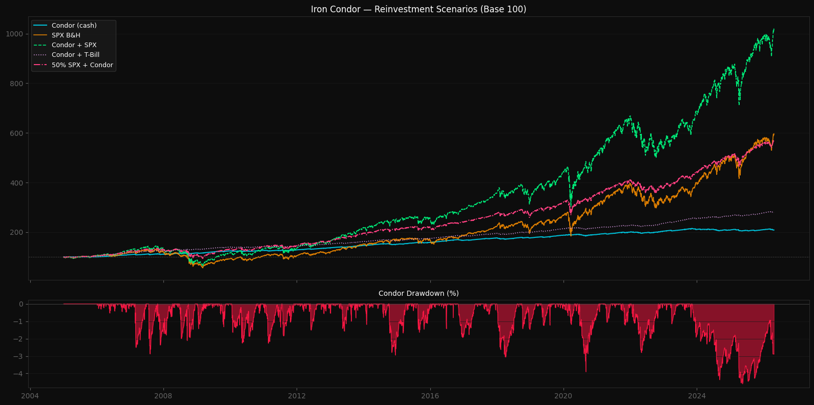
The backtest runs from January 2005 to April 2026 on ES Futures (E-mini S&P 500, $50 multiplier). Every third Friday, a new Iron Condor is opened: a short put spread and a short call spread placed one standard deviation away from the spot price. Wing width is 50 points per side. The position is closed when it reaches 100% of the credit received (take profit). Starting capital is $1,000,000. No stop-loss is applied in the base configuration.

Five portfolio scenarios are compared: the raw Condor cash equity, SPX buy-and-hold, the Condor with profits reinvested in SPX, the Condor with profits compounding at the risk-free rate (IRX), and a 50/50 split between SPX and the Condor.

The raw Condor cash delivers a Sharpe of 1.38 and a Sortino of 1.22 — exceptional risk-adjusted numbers — but a CAGR of only 9.4%. Compounding at the risk-free rate (Condor + IRX) improves the Sharpe to 1.68 and Sortino to 1.46, with a max drawdown of just −9.4%. The most compelling allocation for a practitioner is 50% SPX + Condor: CAGR 14.1%, Sharpe 1.14, Sortino 1.18, max drawdown −28.4%, total return +1539% — against the SPX's +496% with a −57% drawdown.

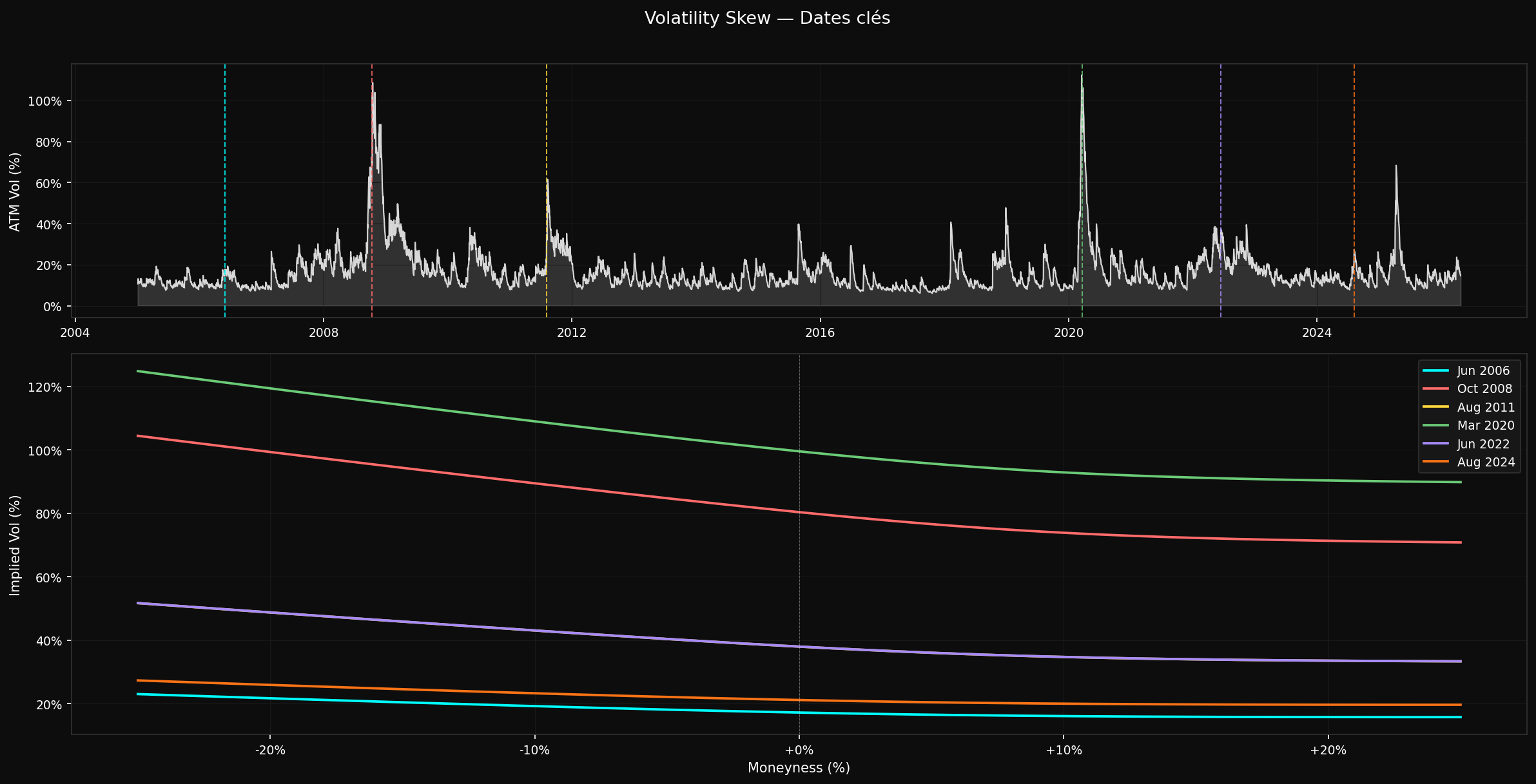
Backtesting an options strategy requires implied volatility data for every strike and every day. That data does not exist for free over 20 years. The solution used here is to reconstruct the surface synthetically: fit a GARCH(1,1) model with Student-t innovations on the daily return series to extract conditional volatility estimates, then generate an SVI (Stochastic Volatility Inspired) smile for each date using regime-dependent parameters. The GARCH model mean-reverts faster than a rolling window — after a spike, it decays toward the long-run mean in days rather than weeks, which makes it a better proxy for what the market would have implied. The Student-t distribution captures the fat tails of daily equity returns, producing better-calibrated vol estimates during the tail events that dominate options P&L.

The SVI parameterization maps log-moneyness to implied variance through five parameters: level (a), slope and curvature (b), correlation between spot and vol (ρ, negative for equity indices — the leverage effect), smile center shift (m), and smoothness (σ). In a crisis regime (GARCH vol > 40%), ρ is pushed to −0.99, the put wing steepens sharply, and the smile minimum shifts into OTM call territory — matching what was actually observed in March 2020 SPX surfaces. In calm regimes, all parameters relax toward a shallow, centered smile.

Two limits are worth being explicit about. First, the volatility skew in the model is too flat. The SVI parameters are set by hand to match the qualitative shape of real surfaces, not calibrated on actual market data. In practice, put skew on ES is significantly steeper than what this model produces — especially in moderate-stress regimes. A steeper put wing means the put spread premium is higher but so is the cost of the long put leg. The net effect on credit collected is ambiguous, but the mark-to-market behavior in a selloff will be worse than the backtest suggests, because the short put will re-price faster than the model assumes.

Second, the VRP is set to zero. In reality, the VRP is positive on average — roughly 3 vol points over the long run. Setting it to zero is conservative: it means option prices in the backtest are lower than what the market would actually have offered. Adding 250 basis points of VRP would make the backtest look better but would also be wrong, because the VRP is variable and sometimes negative. The honest choice is to leave it at zero and acknowledge that real-world results will likely be better in calm regimes and worse in stress.

In production, the strategy runs on three additional layers that the backtest does not capture. First, a systematic entry signal: positions are only opened when implied vol exceeds realized vol by a meaningful margin, and when the market regime is classified as stable (no risk-off signal, no strong trend). Second, dynamic delta hedging: the delta of the book is monitored continuously and rebalanced via ES futures to stay near zero. When a call spread is being tested by the market, the put spread strikes are rolled up to collect additional credit and restore delta neutrality — and vice versa. Third, vega hedging: when implied vol drops sharply after entry, locking in a large portion of the VRP, the position can be partially hedged by buying VIX futures to prevent a sudden vol reversal from reversing the gains. The infrastructure runs on Python with the Interactive Brokers API, using a standalone Black-Scholes IV solver decoupled from the backtesting stack.