Long/Short Trading Explained by a Pro Trader: Profit Regardless of Market Direction
Quant Trading
A complete breakdown of long/short equity strategies as used in institutional trading: mean reversion, relative value, divergence, beta hedging, and two Python backtests — JPMorgan vs Goldman Sachs and SPY vs FEZ. Includes IBKR execution and an honest assessment of the risks nobody talks about.
Antoine
CEO - CodeMarketLabs
2026-05-08
What if you could always be at least half on the right side of the market, regardless of direction? That is exactly what long/short trading is. This article covers everything: the mechanics, the P&L calculation, risk management, and two complete Python backtests — one mean reversion pair (JPMorgan vs Goldman Sachs) and one structural divergence trade (SPY vs FEZ). All code from the accompanying Jupyter Notebook is explained step by step.
What this article covers
What a long/short trade is and why it eliminates directional market exposure.
The three main approaches: mean reversion, relative value, and divergence.
How to calculate a beta hedge ratio using OLS regression and why dollar-neutral is not market-neutral.
Full Python backtest: JPMorgan vs Goldman Sachs — cointegration test, Z-score signals, equity curve.
How to execute a beta-hedged pair trade on Interactive Brokers in two clicks.
Full Python backtest: SPY vs FEZ — structural US/Europe divergence, buy-and-hold spread.
The risks nobody talks about: M&A risk, short financing costs, liquidity, and correlation breakdown.
1. What Is a Long/Short Trade?
A long/short trade is not a directional bet — it is a bet on a differential. Instead of asking whether the market goes up or down, you ask which of two assets will outperform the other. You go long the one you expect to outperform, short the one you expect to underperform, and in doing so you neutralize most of your exposure to the broader market.
The universe of possible pairs is vast. You can trade a differential between two indices, two equities, or two currencies. You can play an index against a sector index — for example the S&P 500 against S&P 500 Technology. You can trade factor against factor, or stocks within the same factor (highest quality vs lowest quality names). You can go long the equity index of an oil-producing country and short the index of a heavy oil consumer, or long a semiconductor-producing nation and short a semiconductor-consuming one. You can build a basket of Goldman Sachs, JPMorgan, and Morgan Stanley versus a basket of regional US retail banks. The range of what is possible in long/short is enormous — and it is one of the most intellectually rich areas of systematic trading, combining quantitative methods, macroeconomic views, and rigorous risk management.
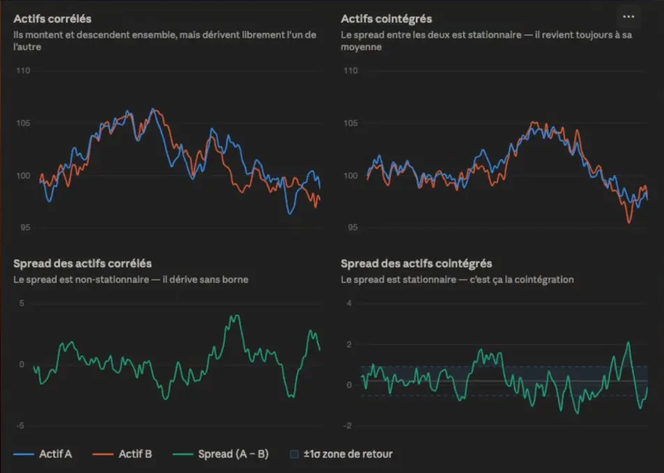
Actifs corrélés vs cointégrés stationnarité du spread pairs trading
2. The Three Main Approaches
There are three distinct ways to structure a long/short trade, each with a different statistical foundation and holding period.
Mean reversion is the most widely discussed approach — and arguably the most difficult to implement correctly. The idea is to find two assets that have historically moved together (same sector, same business lines, same drivers) and trade the spread back to its equilibrium when it deviates abnormally. When the spread widens, you bet on convergence. When it narrows, you bet on re-widening. The key prerequisite is cointegration: not just correlation, but a statistically stable long-run price relationship. Correlation means two assets move in the same direction over a given window. Cointegration means the spread between them is stationary — it fluctuates around a stable mean rather than drifting without bound. Two assets can be highly correlated without being cointegrated, which is exactly why the Engle-Granger test matters before entering any mean reversion trade.
Relative value is simpler in structure: you buy one asset and short another, aiming to capture the outperformance of one over the other. The holding period is typically longer and the thesis is more fundamental. Examples include being long Euro Stoxx 50 and short the Stoxx 600 Autos, long Taiwan (semiconductor producer) vs short South Korea (heavy semiconductor consumer), long India vs short Indonesia, or long S&P 500 vs short S&P 500 Tech. The goal is not mean reversion but pure capture of a structural performance differential — you apply a hedge ratio and hold the spread.
Divergence is the inverse of mean reversion. You identify two assets that have been cointegrated — that is, their spread has historically been stationary — and then you identify a catalyst that should cause that equilibrium to break permanently. Instead of betting on convergence, you bet on the spread widening structurally. The signal can be discretionary or systematic; what matters is having a specific reason to believe the long-run relationship has changed.
3. Beta Hedging: Why Dollar-Neutral Is Not Enough
The most common mistake in pair trading is assuming that buying $100k of one stock and shorting $100k of another produces a market-neutral position. It does not. What matters is not dollar exposure but beta-adjusted exposure. If your long has a beta of 1.2 to the S&P 500 and your short has a beta of 0.8, you are net long the market by a significant margin. Your position has directional risk embedded in it, and in a sell-off you will lose on both sides.
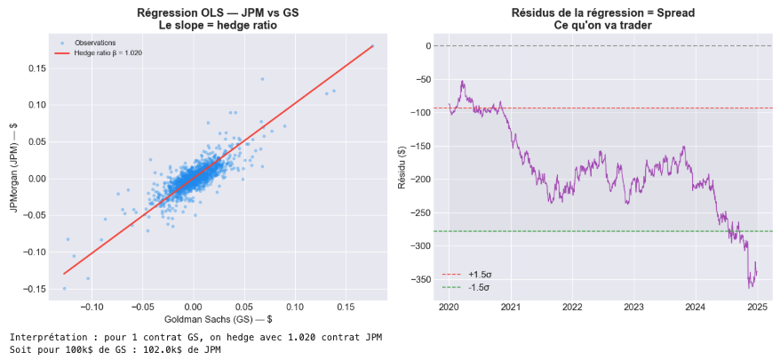
The correct approach is to calculate each asset's beta relative to a reference index (typically the S&P 500 or a sector index) via OLS regression, then compute the hedge ratio as the ratio of the two betas. For JPMorgan vs Goldman Sachs, the calculation produces a hedge ratio of approximately 1.02 — meaning that for every $100k of Goldman Sachs, you need $102k of JPMorgan to be beta-neutral. Because the two banks have very similar market relationships (as expected given their business model overlap), the ratio is close to 1. In pairs with more divergent betas, the ratio can be significantly different from 1, and getting it wrong produces a hidden directional bet that will manifest precisely when you least want it — during a market stress event when correlations spike toward 1.
Régression OLS JPM vs GS hedge ratio et résidus du spread
One important limitation of this approach: the R² of the regression between either stock and the S&P 500 is around 0.50, meaning the beta estimate captures only half of the stock's variance. Beta is not static — it evolves over time, especially during regime changes. For a more robust implementation, beta should be recalculated on a rolling window and the hedge ratio updated periodically. Position-level stops on the spread (not just on the individual legs) and diversification across multiple pairs are additional layers of robustness.
4. Example 1 — Mean Reversion: JPMorgan vs Goldman Sachs
The first backtest implements a mean reversion strategy on JPMorgan and Goldman Sachs from January 2020 to December 2024. Both are large US banks with overlapping business lines, making them natural candidates for a cointegration-based strategy. The methodology follows four steps: download price data and compute returns, run the Engle-Granger cointegration test, compute the OLS hedge ratio and construct the spread, then generate Z-score signals and backtest the P&L.
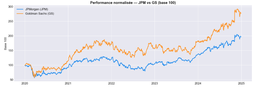
Performance normalisée JPMorgan vs Goldman Sachs base 100
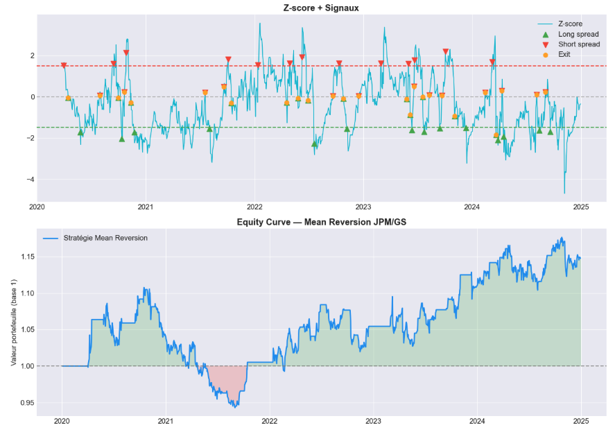
The cointegration test returns a p-value of 0.19 — above the 5% threshold. The pair is not cointegrated over this period. This is an honest result, and it matters: mean reversion on a non-cointegrated pair is not statistically justified. The spread is non-stationary (confirmed by the ADF test), meaning it drifts without a stable mean to revert to. In practice, this pair would be better suited to a divergence trade — simply being long GS vs short JPM — rather than trading the spread symmetrically. The backtest is nevertheless run to completion for educational purposes, with entry at Z-score ±1.5 and exit at 0.
Signaux Z-score et equity curve mean reversion JPMorgan Goldman Sachs
5. Executing a Beta-Hedged Pair on Interactive Brokers
Once the hedge ratio is calculated, executing the trade on Interactive Brokers takes less than a minute. In the TWS terminal, select the long leg (JPM), create a buy order, and choose 'Beta Hedge' from the order type menu. Enter the hedge asset (GS), set the beta ratio (1.02), and set the max hedging size. IBKR automatically calculates the offsetting short order on Goldman Sachs and routes both legs simultaneously. The result is a position where the market value of the short leg slightly exceeds the long leg — by exactly the hedge ratio — producing a beta-neutral book. The same logic applies to algorithmic execution via the IBKR API, where the hedge ratio computed in Python feeds directly into the order parameters.
6. Example 2 — Relative Value: SPY vs FEZ (US vs Europe)
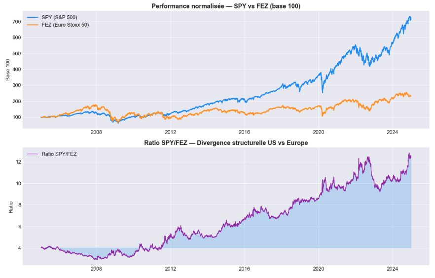
The second example is the purest form of relative value: long SPY (S&P 500) and short FEZ (Euro Stoxx 50), held permanently. There is no Z-score, no entry signal, no mean reversion thesis. The trade expresses a single structural conviction: US equities generate higher returns than European equities over time, driven by stronger shareholder return culture, higher corporate profitability targets, less regulatory burden, and a more dynamic capital allocation machine.
Performance normalisée SPY vs FEZ divergence structurelle US Europe ratio
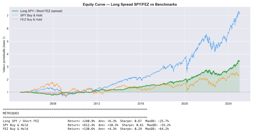
The backtest runs from January 2005 to December 2024 with $100k on each leg. Metrics: Long SPY / Short FEZ delivers +240.9% total return, annualized at +6.3%, Sharpe 0.67, max drawdown −25.7%. SPY buy-and-hold delivers +612.4% with a max drawdown of −55.2%. The spread strategy has a significantly lower absolute return than outright SPY — that is expected, since you are shorting part of the market's upside. The value is in the risk profile: the max drawdown is less than half of SPY's, and the equity curve is far smoother. The practical extension of this trade is to combine it with a long position in the underlying market: hold SPY directly and express the relative trade via futures (long ES, short EuroStoxx futures) without deploying additional capital. The combined position captures both the SPX beta and the spread, historically outperforming the index on a risk-adjusted basis.
Equity curve long SPY short FEZ vs benchmarks relative value long short
7. The Risks Nobody Talks About
Long/short strategies have a specific risk profile that is rarely covered in textbooks and often learned the hard way on live markets.
On single-stock pairs, the most dangerous risk is M&A. If you are long JPMorgan and short Goldman Sachs, and JPM announces a takeover bid for GS, you face a catastrophic loss: JPM drops on the capital outflow from funding the acquisition, while GS spikes on the bid premium. Before entering any single-stock pair, conduct due diligence on the ownership structure of both names. A stock with a family or controlling shareholder holding 40% is a potential going-private candidate. A stock with highly fragmented institutional ownership is less vulnerable. This check is non-negotiable.
The second risk is correlation breakdown in crisis regimes. In a market stress event, nearly everything becomes correlated near 1 on the downside. If your hedge ratio is below 1, your long leg loses more than your short leg gains, and you realize a directional loss that your model did not anticipate. This is the gap between modeled cointegration and what actually materializes in a tail event. It is not a model failure — it is a known property of financial markets that needs to be managed with position-level stops on the spread, not just on the legs.
The third risk is the cost of carrying a short position. Shorting a stock is not free — the borrowing cost ranges from a few basis points annually for large liquid names to 50 basis points, 1%, or even 2% per month for small, illiquid stocks. The smaller and less liquid the stock, the more expensive the short. This cost must be explicitly modeled in the backtest as an annualized rate applied to the short leg's notional. Failing to do so produces backtest results that cannot be replicated in production. Related to this: liquidity itself is a risk on small-cap names. Thin markets can produce outsized moves on entry and exit, making the theoretical spread untradeable in practice. Build your tradeable universe around mid-cap and large-cap names with stable liquidity profiles, and on the futures side, avoid contracts with low open interest or no volume — they exist on IBKR but cannot be traded at fair value.
What the Notebook contains
Part 1 — JPM vs GS: full data pipeline, Engle-Granger cointegration test, OLS hedge ratio, ADF test on the spread, Z-score signal generation, backtest engine, equity curve with entry/exit markers.
Part 2 — SPY vs FEZ: data download, normalized performance and ratio chart, fixed-notional P&L computation, equity curve vs benchmarks, full metrics (CAGR, Sharpe, max drawdown).
Metrics function reusable across any pair: total return, annualized return, Sharpe ratio, max drawdown.
Clean matplotlib visualizations formatted for direct use in articles and presentations.
What is the difference between correlation and cointegration?
Correlation measures whether two assets move in the same direction over a given time window. Cointegration is a stronger condition: it means the spread between the two assets' prices is stationary — it fluctuates around a stable mean and tends to revert to it. Two assets can be highly correlated without being cointegrated (they move together but drift apart over time). For mean reversion trading, cointegration is what matters, not correlation. The Engle-Granger test checks whether the spread is stationary by running an ADF test on the regression residuals.
Why is dollar-neutral not the same as market-neutral?
Dollar neutrality means equal notional on each leg. Market neutrality means equal beta-adjusted exposure. If your long stock has a beta of 1.3 and your short has a beta of 0.7, a dollar-neutral position is still net long the market by 0.6 beta. In a sell-off, your long leg loses more than your short leg gains, and you realize a directional loss. The correct approach is to size the legs so that beta × notional is equal on both sides — which almost always means unequal dollar amounts.
When should you use mean reversion vs relative value vs divergence?
Mean reversion requires a statistically validated cointegration relationship — confirmed by a p-value below 5% on the Engle-Granger test. It is appropriate when two assets have a demonstrated tendency for their spread to revert to a stable level. Relative value is appropriate when you have a fundamental conviction about structural outperformance of one asset over another, without expecting the spread to revert. Divergence is the mirror of mean reversion: you identify a previously cointegrated pair and bet that a fundamental shift will cause the spread to widen permanently.
How do you handle the M&A risk on a short position?
Before entering any single-stock short, check the ownership structure. A company with a controlling family shareholder, a private equity backer with a large stake, or an activist investor accumulating a position is a potential M&A or going-private candidate. If a takeover bid is announced on your short, the stock can gap 20–40% overnight and your position is immediately deeply underwater. The practical mitigation is to avoid stocks with concentrated ownership on the short side, to run stops on the spread (not just the individual legs), and to diversify across enough pairs that any single M&A event does not threaten the overall book.
Can this strategy be run on a small retail account?
The mean reversion strategy on equities (JPM/GS) requires a margin account and short-selling capability — available on Interactive Brokers even for retail clients. The relative value strategy via ETFs (SPY/FEZ) can also be run in a standard margin account. The futures version (long ES / short EuroStoxx) requires futures approval and a minimum account size to make the hedge sizes meaningful, since one ES contract represents $50 × the index level. For smaller accounts, the ETF version is the practical entry point.
How often should you recalculate the hedge ratio?
Beta is not constant — it evolves with market regimes, especially during stress events. A static hedge ratio computed on a full historical window will lag the current market relationship. A reasonable approach is to recalculate the hedge ratio on a rolling 60-day or 120-day window and update the position accordingly. More frequent rebalancing captures regime shifts faster but generates more transaction costs. The right frequency depends on the turnover and holding period of the strategy.