Quantkit: A Python Library for Derivatives Pricing, Volatility Modeling, and Rates Analysis
Tools Documentation
quantkit is a Python library for quantitative analysts and derivatives traders. It covers the full pricing stack — seven stochastic models calibrated via FFT on real options surfaces, a complete Black-Scholes Greeks engine, multi-leg portfolio management with interactive dashboards, and a rates toolkit spanning Nelson-Siegel, Hull-White, and Vasicek models.
Antoine
CEO - CodeMarketLabs
2026-03-20
quantkit: A Python Library for Derivatives Pricing, Volatility Modeling, and Rates Analysis
quantkit is a professional-grade Python library built for quantitative analysts, derivatives traders, and portfolio managers who need a rigorous, modular framework spanning the full pricing stack. It covers three distinct domains in a unified codebase: stochastic model calibration on real options surfaces, multi-leg options strategy management with a complete Greeks engine, and interest rate curve modeling from parametric fitting to short-rate simulation. Every module is independently usable — calibrate a single model, compute a Greek surface, or run a full interactive dashboard from one line.
What the library provides
Seven stochastic models with FFT-based pricing: Heston, Bates, Variance Gamma, Merton, Kou, NIG, CGMY — calibrated via Latin Hypercube search and SLSQP optimisation.
Full Black-Scholes Greeks engine: 18 sensitivities from Delta to Ultima, computed analytically across any multi-leg portfolio.
DerivativesPortfolio class: build any multi-leg structure, compute Greeks, run Monte Carlo simulations, and generate interactive dashboards.
Interest rate curves: four parametric models (Nelson-Siegel, NSS, Bjork-Christensen, BCA) and two stochastic models (Hull-White, Vasicek) with Plotly visualisation.
Futures curve support: each option maturity maps to its correct underlying futures contract — no synthetic forward approximation.
Exotic derivatives pricing via Monte Carlo: vanilla, Asian, barrier, lookback, range accrual, digital, variance swap, and Phoenix autocall.
1. Stochastic Models and FFT Calibration
The calibration engine prices options via the Fast Fourier Transform using the characteristic function of each model. This makes it possible to evaluate thousands of (strike, maturity) pairs simultaneously, which is a prerequisite for fitting a full volatility surface in reasonable time. The starting point search uses a Latin Hypercube Sampler to cover the parameter space efficiently before handing off to SLSQP with model-specific bounds. Each model exposes a set_all_params method, a phi (characteristic function), simulate_paths, and print_model — providing a consistent interface regardless of which model is in use.
python
import src.quantkit.stochastics.calibration as cal
import src.quantkit.stochastics.models as mod
from src.quantkit.rates.utils.curve import Curve, FuturesCurve
from src.quantkit.rates.curve_interpolation.bjork_christensen_augmented import BjorkChristensenAugmented
import numpy as np
from datetime import datetime
# --- Rate curve: calibrate BCA on SOFR data ---rates =[(datetime(2026,3,19),3.67),(datetime(2026,5,19),3.68),(datetime(2026,6,22),3.64),(datetime(2026,7,20),3.61),(datetime(2026,10,19),3.5),(datetime(2026,11,19),3.47),(datetime(2026,12,21),3.45)]today = datetime(2026,3,20)rates_mat = np.array([(d - today).days /365for d, _ in rates])rates_val = np.array([r /100for _, r in rates])bca = BjorkChristensenAugmented(beta0=4.0, beta1=-0.5, beta2=-1.0, beta3=0.5, beta4=0.3, tau=3.0)bca.calibrate(Curve(rates_mat, rates_val))# --- Futures curve: maps each option maturity to the correct futures contract ---futures =[(datetime(2026,6,19),6670.25),(datetime(2026,9,18),6711),(datetime(2026,12,18),6835)]futures_exp = np.array([(d - today).days for d, _ in futures])futures_curve = FuturesCurve(futures_exp, np.array([p for _, p in futures]))spot = futures_curve.yield_t(0)# first futures price as spot# --- Heston model: calibrate on the call surface ---model = mod.HestonModel( spot_zero=spot, rfr=0.035, div=0.01, tt_maturity=1, kappa=1.5, theta=0.04, vol_vol=0.3, rho=-0.7, vol_zero=0.04)alpha, eta, n =-2,0.1,12rmse_array, best_start = cal.find_starting_point( model, call_surface, bca, bca, alpha, eta, n,"call", n_points=100, futures_curve=futures_curve
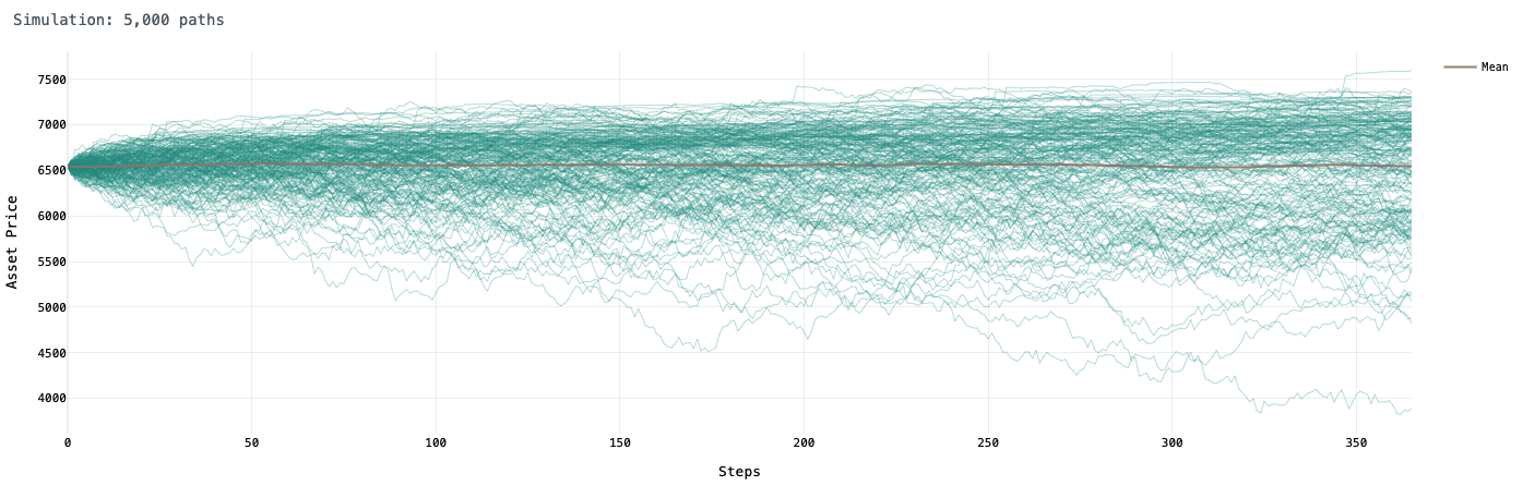
)args =(model, call_surface, bca, bca, alpha, eta, n,"call",1, futures_curve)result = cal.calibration(best_start.tolist(), args, method="SLSQP")print(f"RMSE: {result.fun:.4f} | Converged: {result.success}")# --- Simulate paths from the calibrated model ---sim = model.simulate_paths(n_paths=5000, divider=365)sim.plot(max_paths=450)
Simulation Monte Carlo — 5 000 chemins sur un an sous le modèle de Bates calibré, avec le chemin moyen en superposition.
2. The Seven Models
Each model addresses a different aspect of the observed volatility smile. Heston introduces stochastic variance with mean reversion, producing a smooth smile that fades slowly across maturities. Bates extends Heston with compound Poisson jumps, allowing simultaneous fit of the volatility surface and the left tail — the most flexible standard model for equity indices. Variance Gamma is a pure jump process driven by a Gamma-subordinated Brownian motion, capturing skewness and excess kurtosis with just three parameters. Merton is the classic jump-diffusion baseline: simple, interpretable, and fast. Kou replaces Gaussian jumps with a double exponential distribution, giving fatter tails and closed-form barrier pricing. NIG and CGMY are infinite-activity Lévy processes — NIG is analytically tractable and widely used in energy markets, while CGMY's Y parameter controls the fine structure of small jumps from finite to infinite activity.
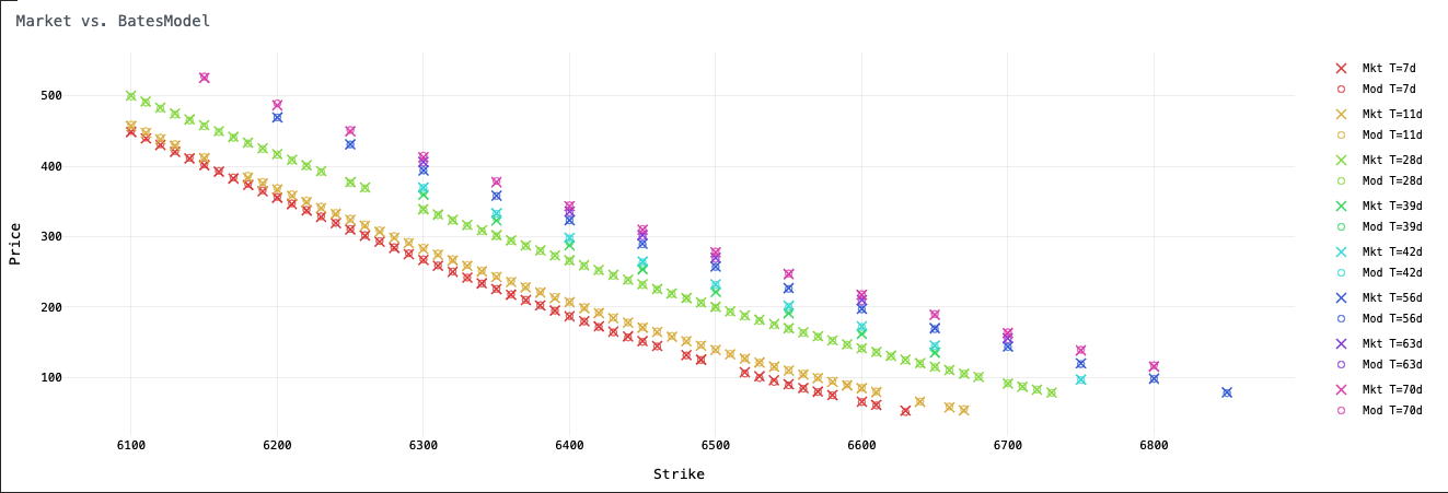
Calibration du modèle de Bates sur la surface d'options SPX — prix marché (×) vs prix modèle (○) sur sept maturités de 7 à 70 jours.
3. Monte Carlo Pricing — Vanilla and Exotic Derivatives
Once a model is calibrated, simulate_paths returns a Simulation object containing the full price matrix. Every exotic payoff is then a vectorised numpy operation over the terminal or path-wise prices. The same simulation block prices all instruments simultaneously — one model run, any number of products. The framework handles path-dependent payoffs naturally: barrier monitoring is a single any() call across the path axis, Asian averaging is mean() along the time axis, and the Phoenix autocall loop iterates over quarterly observation dates while tracking which paths are still alive.
python
# Calibrate Merton, simulate paths, price everything in one passmodel_bates = mod.Merton( spot_zero=spot, rfr=0.035, div=0.01, tt_maturity=1, sigma=0.2, lamb=0.75, mu_j=-0.23, sig_j=0.05)# ... calibrate as above ...x = model_bates.simulate_paths(5000,365)terminal = x.paths[-1,:]paths = x.paths
T, rfr_ = model_bates.tt_maturity, model_bates.rfr
df = np.exp(-rfr_ * T)S0, K = model_bates.spot_zero,7000# Vanillapayoff_call = np.maximum(terminal - K,0)payoff_put = np.maximum(K - terminal,0)print(f"Call K={K} : {df * np.mean(payoff_call):.2f}")print(f"Put K={K} : {df * np.mean(payoff_put):.2f}")print(f"Straddle : {df * np.mean(payoff_call + payoff_put):.2f}")# Asian call (arithmetic average)print(f"Asian Call : {df * np.mean(np.maximum(paths.mean(axis=0)- K,0)):.2f}")# Knock-out call (barrier at 7500)knocked_out = np.any(paths >7500, axis=0)print(f"KO Call B=7500 : {df * np.mean(np.where(knocked_out,0, np.maximum(terminal - K,0))):.2f}")# Knock-in put (barrier at 6000)knocked_in = np.any(paths <6000, axis=0)print(f"KI Put B=6000 : {df * np.mean(np.where(knocked_in, np.maximum(K - terminal,0),0)):.2f}")# Lookback callprint(f"Lookback Call : {df * np.mean(np.maximum(terminal - paths.min(axis=0),0)):.2f}")# Digital callprint(f"Digital B=8000 : {df * np.mean(np.where(terminal >8000,1000,0)):.2f}")# Range accrual — pays 1000/365 per day S stays in [6000, 7500]in_range =(paths >=6000)&(paths <=7500)print(f"Range Accrual : {df * np.mean(in_range.sum(axis=0)*1000/365):.2f}")
4. Exotic Derivatives Pricing
The same simulation block prices every product simultaneously — one calibrated model, one simulate_paths call, any number of instruments. Digital options price the risk-neutral probability of an event directly. Barrier options (knock-out and knock-in) monitor the full path using a single vectorised any() call. Asian options average the path arithmetically. Lookback options use the floating minimum as a strike. Range accruals count the days the underlying stays within a corridor. Every payoff is a few lines of numpy — no numerical integration, no PDE solvers.
python
# All payoffs computed from the same simulation — one pass, many productsx = model_bates.simulate_paths(5000,365)terminal = x.paths[-1,:]paths = x.paths
T, rfr_ = model_bates.tt_maturity, model_bates.rfr
df = np.exp(-rfr_ * T)S0, K = model_bates.spot_zero,7000# Digital call — pays 1000 if S(T) > 8000, else 0payoff_digital = np.where(terminal >8000,1000,0)price_digital = df * np.mean(payoff_digital)prob_above = np.mean(terminal >8000)print(f"Digital Call B=8000 price: {price_digital:.2f} | risk-neutral prob: {prob_above*100:.1f}%")# Knock-out call — barrier kills the option if S ever exceeds 7500knocked_out = np.any(paths >7500, axis=0)payoff_ko = np.where(knocked_out,0, np.maximum(terminal - K,0))print(f"KO Call K=7000 B=7500 : {df * np.mean(payoff_ko):.2f}")# Knock-in put — only activates if S ever drops below 6000knocked_in = np.any(paths <6000, axis=0)payoff_ki = np.where(knocked_in, np.maximum(K - terminal,0),0)print(f"KI Put K=7000 B=6000 : {df * np.mean(payoff_ki):.2f}")# Asian call — strike vs arithmetic average of the pathpayoff_asian = np.maximum(paths.mean(axis=0)- K,0)print(f"Asian Call K=7000 : {df * np.mean(payoff_asian):.2f}")# Lookback call — floating strike = minimum realised pricepayoff_lb = np.maximum(terminal - paths.min(axis=0),0)print(f"Lookback Call : {df * np.mean(payoff_lb):.2f}")# Range accrual — pays 1000/365 per day S stays inside [6000, 7500]in_range =(paths >=6000)&(paths <=7500)payoff_ra = in_range.sum(axis=0)*(1000/365)print(f"Range Accrual [6k,7.5k]: {df * np.mean(payoff_ra):.2f}")# Vanilla referencepayoff_call = np.maximum(terminal - K,0)payoff_put = np.maximum(K - terminal,0)print(f"Vanilla Call K=7000 : {df * np.mean(payoff_call):.2f}")print(f"Vanilla Put K=7000 : {df * np.mean(payoff_put):.2f}")print(f"Straddle : {df * np.mean(payoff_call + payoff_put):.2f}")
5. DerivativesPortfolio and Greeks Engine
DerivativesPortfolio is the portfolio management layer. It accepts long and short positions in calls, puts, spot, and futures through a clean fluent interface and stores each leg internally. The Greeks engine uses closed-form Black-Scholes analytical formulas for 18 sensitivities — from first-order (Delta, Vega, Theta, Rho) through second-order (Gamma, Vanna, Vomma, Charm) to third-order (Speed, Zomma, Color, Ultima). Each Greek is weighted by net quantity and aggregated at the portfolio level. The compute_greeks method accepts per-leg implied volatilities, dividend rates, and risk-free rates, so a realistic skew structure can be represented directly.
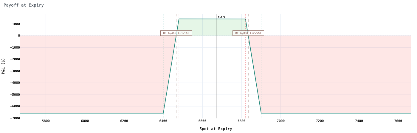
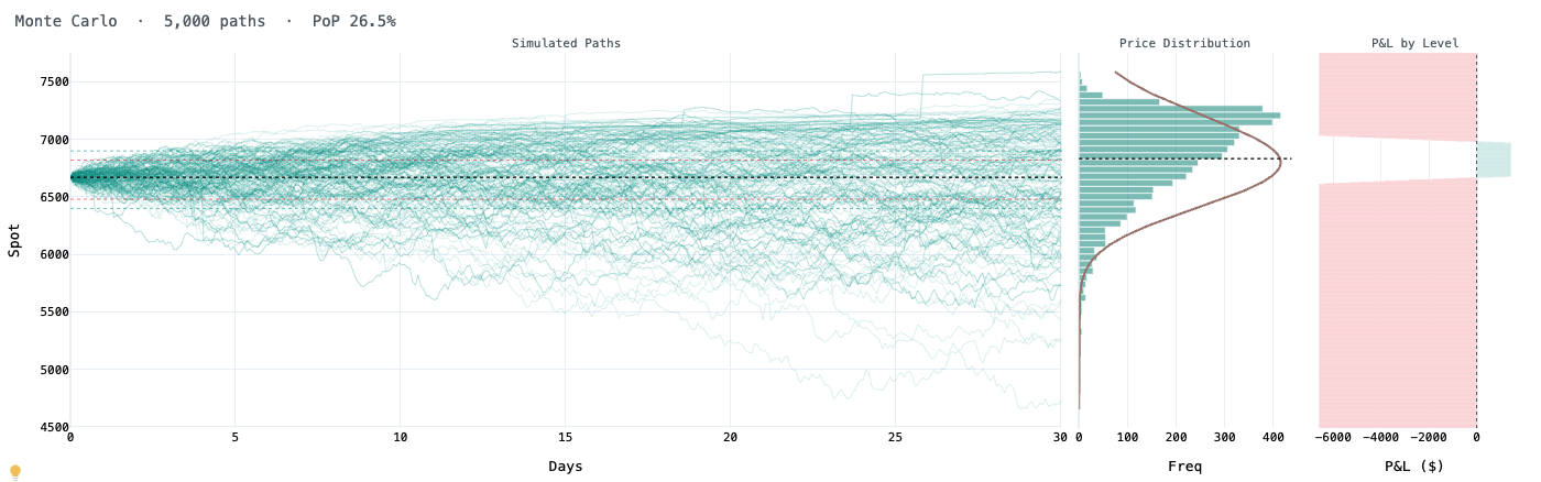
Payoff à l'expiration d'un Iron Condor sur ES — break-evens à 6 466 (-3,1%) et 6 834 (+2,5%), spot courant à 6 670.Panel Monte Carlo — chemins simulés, distribution des prix terminaux et P&L ladder pour un Iron Condor, avec une probabilité de gain de 26,5%.
6. Interactive Dashboards
The graphs module provides standalone Plotly figures for every analytics dimension and a dashboard function that assembles all of them into a single scrollable figure. The layout covers payoff diagrams with break-even annotations, Monte Carlo path simulations, terminal price and P&L distributions, a vol/spot sensitivity heatmap, individual Greek profiles as functions of spot, vol, or time, 3D MTM and Delta surfaces, and summary statistics tables. Dark and light themes are supported throughout. The dashboard renders in Jupyter notebooks or exports to a self-contained HTML file or PNG.
Dashboard complet d'un Broken Wing Butterfly sur ES Jun26 — payoff, Greeks, stress test, Monte Carlo, distribution P&L, profils de Greeks et surfaces 3D.
7. Interest Rate Curve Modeling
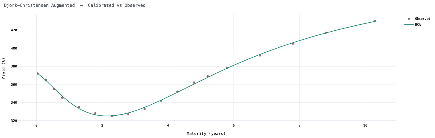
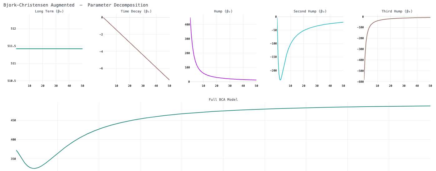
The rates module provides a complete term structure toolkit. On the interpolation side, LinearCurve and CubicCurve wrap scipy interpolators with a consistent d_rate / df_t / forward interface. On the parametric side, four models are available: Nelson-Siegel (3 factors), Nelson-Siegel-Svensson (4 factors with a second hump), Bjork-Christensen (alternative second factor for better short-end fit), and Bjork-Christensen Augmented (5 factors including a linear drift term). All four share the same calibrate / d_rate / df_t / forward_rate / plot_* interface and are calibrated via L-BFGS-B minimisation of squared errors on observed zero rates. Each model produces five Plotly charts: calibrated vs observed, component breakdown, parameter decomposition subplots, discount factor term structure, and spot vs forward curve.
Modèle Bjork-Christensen Augmenté calibré sur la structure de terme SOFR — taux zéro observés (points) vs courbe fittée (ligne) de 0 à 10 ans, capturant l'inversion en U avec un creux autour de 2,5 ans.Bjork-Christensen Augmenté — décomposition des cinq facteurs : niveau long terme (β₀), dérive linéaire (β₁), bosse (β₂), deuxième bosse (β₃), troisième bosse (β₄), et la courbe BCA complète résultante sur un horizon de 50 ans.
8. Stochastic Rate Models — Hull-White and Vasicek
The stochastic rates module provides two short-rate models. Vasicek is the original affine mean-reverting model with constant parameters and closed-form zero coupon bond prices — analytically tractable but structurally limited to monotone term structures. Hull-White is the time-dependent extension: the drift theta(t) is inferred from the initial yield curve via a Pchip spline on log discount factors, allowing the model to fit any initial curve exactly by construction. Hull-White is the standard model for interest rate derivatives pricing — callable bonds, bermuda swaptions, and rate-sensitive structured products require consistent path simulation, which Vasicek's monotone constraint makes impossible on real market curves. Both models use Euler-Maruyama simulation and expose calibrate, simulate_paths, and plot_* methods.
python
from src.quantkit.rates.stochastics.hull_and_white import HullWhite
from src.quantkit.rates.stochastics.vasicek import Vasicek
import numpy as np
# --- Hull-White on the U-shaped SOFR curve ---hw = HullWhite(a=0.1, sigma=0.01, curve=curve)# curve = SOFR Curve object from abovehw.calibrate()# calibrates a and sigma; theta(t) is computed analyticallyhw.print_model()hw.plot_calibrated(mode='dark').show()# zero rate fithw.plot_term_structure(mode='dark').show()# zero + forward curvehw.plot_simulated_paths(n_paths=500, n_steps=252, T=10.0, n_show=200, mode='dark').show()paths_hw = hw.simulate_paths(n_paths=50000, n_steps=252, T=10.0)terminal_hw = paths_hw[-1,:]*100print(f"Mean terminal rate : {terminal_hw.mean():.3f}%")print(f"Std terminal rate : {terminal_hw.std():.3f}%")print(f"P(r < 0) : {(terminal_hw <0).mean()*100:.2f}%")# VaR on a 10Y futures — use the Hull-White sigma from market swaption volvol_atm_10y =0.0080# 80 bps annualised — replace hw.sigma to make market-consistenthw_var = HullWhite(a=hw.a, sigma=vol_atm_10y, curve=curve)paths_var = hw_var.simulate_paths(n_paths=50000, n_steps=10, T=10/252)r_terminal = paths_var[-1,:]# short rate at T+10 daysf0_10y = hw._f_mkt(10.0)# instantaneous forward at 10yB =(1- np.exp(-hw.a *10.0))/ hw.a
r10y_paths =(f0_10y +(r_terminal - f0_10y)* B /10.0)*100dv01 =0.09*100000/100pnl =(hw._f_mkt(10.0)*100- r10y_paths)*100* dv01
print(f"VaR 1% (10d) : ${np.percentile(pnl,1):,.0f}")print(f"VaR 5% (10d) : ${np.percentile(pnl,5):,.0f}")# --- Vasicek on a monotone curve (its correct domain) ---curve_mono = Curve(t, np.array([3.5,3.6,3.65,3.8,3.9,3.95,4.0,4.05,4.1,4.15,4.25,4.4,4.5,4.6,4.75,4.85,4.9,5.0]))vasicek = Vasicek(a=0.3, b=0.05, sigma=0.01, r0=float(curve_mono.rt[0])/100)vasicek.calibrate(curve_mono)vasicek.plot_calibrated(curve_mono, mode='dark').show()vasicek.plot_term_structure(mode='dark').show()vasicek.plot_simulated_paths(n_paths=500, n_steps=252, T=30.0, n_show=200, mode='dark').show()
9. Black-Scholes Pricing and Implied Volatility
The options module provides the analytical Black-Scholes engine used internally by DerivativesPortfolio. BsParams is a frozen dataclass that validates all inputs at construction time — invalid option type, negative vol, or non-positive spot or strike will raise immediately. The pricing function handles both calls and puts via the standard d1/d2 formulation with continuous dividends. Put-call parity conversions are available as call_from_put and put_from_call. Implied volatility is solved via bisection — the solver converges to 1e-15 absolute error. All 18 Greeks are available as standalone functions or via the option_carac aggregator which returns a complete dict.
python
from src.quantkit.options.black_scholes_params import BsParams
from src.quantkit.options.pricing import option_price, call_from_put, put_from_call
from src.quantkit.options.greeks import option_carac, delta, gamma, vega, theta, vanna
from src.quantkit.options.iv_solver import implied_vol
# --- Vanilla pricing ---params = BsParams( opt_type='c', volatility=0.20, time_maturity=30/365, risk_free_rate=0.035, dividend=0.011, spot=6670.0, strike=6700.0)print(f"Call price : {option_price(params):.4f}")print(f"Put via PCP : {put_from_call(params, option_price(params)):.4f}")# --- Full Greeks ---g = option_carac(params, side=1)# side=1 long, side=-1 shortfor name, val in g.items():print(f" {name:12s}: {val:.6f}")# --- Implied volatility (bisection, 1e-15 convergence) ---market_price =25.0iv = implied_vol(params, market_price)print(f"\nImplied vol for market price {market_price}: {iv:.4f}")# --- Per-leg greeks without building a full portfolio ---print(f"Delta : {delta(params, side=1):.4f}")print(f"Gamma : {gamma(params, side=1):.6f}")print(f"Vega (1%) : {vega(params, side=1):.4f}")print(f"Theta/day : {theta(params, side=1):.4f}")print(f"Vanna : {vanna(params, side=1):.6f}")
10. Live Market Data Integration via marketconnect-exec
quantkit integrates directly with the marketconnect-exec library to pull live data from Interactive Brokers. The calibration workflow can be fully automated: fetch the futures chain to build the spot and futures curve, fetch the SOFR futures chain to construct the rate curve, pull the live options surface with bid-ask filtering and strike range constraints, and feed all three objects directly into the calibration engine. This closes the loop between live market data and model calibration without any manual data transformation.
python
from marketconnect_exec.brokers.ibkr.adapter import IBKRAdapter
from marketconnect_exec.static.brokers import BrokerName
from marketconnect_exec.exec.execution import Execution
from marketconnect_exec.exec.router import APIRouter
import nest_asyncio
nest_asyncio.apply()# required in Jupyter# --- Connect to IBKR ---router = APIRouter()router.register_broker(IBKRAdapter(port=7496, testnet=False))router.connect_all_brokers()executor = Execution(router)# --- Futures chain → spot and FuturesCurve ---futures_raw = executor.get_futures_chain(BrokerName.IBKR,649180695)# ES contract IDfutures =[(f['expiration'], f['mark_price'])for f in futures_raw ifnot np.isnan(f.get('mark_price', np.nan))]# --- SOFR futures → rate curve ---rates_raw = executor.get_futures_chain(BrokerName.IBKR,385575904)# SOFR futures IDrates =[(f['expiration'],100- f['mark_price'])for f in rates_raw ifnot np.isnan(f.get('mark_price', np.nan))]# --- Options surface with quality filters ---surface = executor.get_vol_surface( BrokerName.IBKR,649180678,# SPX options ID strike_range=(6100,7100), maximum_days=365, filter_bid_ask=True, filter_bid_ask_pct=0.01, surface_type='all', strike_increment=10)# --- Save and proceed with calibration ---import pandas as pd
df_surf = pd.DataFrame(surface)df_surf.to_csv('data_options.csv', index=False)# The rest of the calibration pipeline is identical to the CSV pathrouter.disconnect_all_brokers()
Get quantkit
quantkit is available as a standalone Python package. Whether you are calibrating stochastic models on live options data, managing a multi-leg derivatives portfolio, building structured product pricing tools, or constructing and simulating interest rate curves, the library provides a production-ready analytical stack with a consistent, well-documented API across all modules.
What you get
Full source code: seven stochastic models, FFT calibration engine, complete Greeks, rates toolkit, and interactive dashboards.
Live data integration: direct connectivity to Interactive Brokers via marketconnect-exec for automated surface calibration.
Consistent interface: every model — equity or rates, parametric or stochastic — shares the same calibrate / simulate / plot pattern.
Production-ready charts: dark and light Plotly dashboards exportable to HTML and PNG.
Lifetime updates — new models, products, and features added regularly.
Which stochastic models are included and how do I choose between them?
Seven models are available: Heston, Bates, Variance Gamma, Merton, Kou, NIG, and CGMY. For equity indices with a pronounced skew, Bates is typically the best starting point — it combines stochastic volatility with jump risk. Heston alone fits the smile shape but struggles with the left tail. Pure jump models (VG, NIG, CGMY) fit short-dated smiles well and are useful when you want to avoid the Brownian motion assumption. Merton and Kou are simpler jump-diffusion models — fast, interpretable, and good for teaching or when computation time is limited. All seven share the same calibration interface, so comparison is straightforward.
How does the FFT calibration engine work?
Option prices are computed via the Carr-Madan FFT method: for a given model, the characteristic function phi is evaluated on a grid of log-strike frequencies, multiplied by a damping factor, and inverse Fourier transformed to produce a price surface over a range of strikes simultaneously. This is orders of magnitude faster than evaluating each strike individually. The objective function minimises the relative RMSE between model and market prices across all selected maturities and strikes. A Latin Hypercube sampler finds a good starting point before SLSQP refines the solution with model-specific parameter bounds.
How does the futures curve work, and why does it matter for calibration?
The FuturesCurve object maps each option maturity to the first futures contract expiring after it — the actual deliverable underlying. When you use it in calibration, the spot_zero for each maturity is set to the observed futures price rather than a synthetic forward computed as S * exp((r-q)*T). This matters because the market prices futures directly, and any basis between the synthetic forward and the quoted futures price would otherwise pollute the model parameters. With the futures curve, the drift is absorbed by the futures price itself, and the model parameters focus purely on fitting the volatility smile.
Can I calibrate on put options instead of calls?
Yes. The calibration engine accepts an opt_type parameter set to 'call' or 'put'. In practice, calibrating on calls and puts separately and comparing the resulting parameters is a useful consistency check. For liquid equity index options, both should produce similar parameters because put-call parity holds tightly. For markets with less liquid puts or significant skew, calibrating on out-of-the-money options of each type separately gives better coverage of the smile.
What Greeks does the engine compute, and are they analytical or numerical?
The engine computes 18 Greeks analytically using closed-form Black-Scholes formulas: Delta, Vega, Rho, Theta, Epsilon, Omega (first order), Gamma, Vanna, Vomma, Charm, Veta, Vera (second order), and Speed, Zomma, Color, Ultima (third order). All are analytical — no finite difference approximations. Each Greek function accepts a BsParams object and a side parameter (1 for long, -1 for short). The option_carac aggregator returns all 18 in a single dict, which DerivativesPortfolio uses to aggregate across legs.
What is the difference between Hull-White and Vasicek, and when should I use each?
Vasicek has a constant long-run mean b and can only produce monotone term structures — rates converge smoothly toward b from any initial level. It has closed-form bond prices and is analytically tractable, but it cannot fit a U-shaped or humped yield curve. Hull-White extends Vasicek with a time-dependent drift theta(t) that is inferred analytically from the initial yield curve, allowing it to fit any observed term structure exactly by construction. Use Vasicek for teaching, theoretical exploration, or any situation where a simple parametric model suffices. Use Hull-White whenever you need to simulate rate paths that are consistent with today's observed yield curve — callable bonds, bermuda swaptions, rate-linked structured products, or VaR scenarios.
How do I price exotic derivatives like digitals or barrier options?
Calibrate your model on the options surface, call simulate_paths to get the full price matrix, then implement the payoff as vectorised numpy operations. The Simulation object contains a paths array of shape (n_steps+1, n_paths). A digital is np.where(terminal > B, N, 0). A knock-out barrier is np.any(paths > B, axis=0) followed by masking. An Asian is paths.mean(axis=0). Each product is independent — all are evaluated in a single pass over the same simulation, so pricing ten instruments costs the same as pricing one.
Does quantkit support options on futures, or only options on spot?
Options on futures are fully supported via the FuturesCurve class. When calibrating options on futures, pass a FuturesCurve to the calibration engine. Each option maturity is mapped to the nearest futures contract expiring after it — so an option expiring in 30 days maps to the front-month futures, not to a synthetic spot. The FFT engine sets spot_zero to the relevant futures price and neutralises the drift by setting div equal to rfr, which is equivalent to pricing under the forward measure.
Can I use the rate curve models as discount curves in the options calibration?
Yes, and this is the recommended approach. The calibration engine accepts any object with a d_rate method — LinearCurve, CubicCurve, NelsonSiegel, NelsonSiegelSvensson, BjorkChristensen, or BjorkChristensenAugmented. Calibrate the rate model on observed market rates first, then pass it as both market_rates and market_div to the calibration engine. When combined with a FuturesCurve, the drift and discount factors are both fully market-consistent: rates come from the calibrated curve, and the futures price handles the spot-forward relationship.
What data format does the calibration engine expect for the options surface?
The engine expects a CleanSurface object, which wraps a DataFrame with three columns: times (integer days to expiry), strikes (float), and prices (float mid prices). The standard workflow is: load bid and ask prices, compute the mid, compute time to expiry in days, filter out contracts with missing implied vol or bid/ask, then pass the filtered DataFrame to CleanSurface. The calibration notebook includes the complete data cleaning pipeline for both live IBKR data and CSV files.